$\gdef\e{\mathrm{e}}\gdef\d{\mathrm{d}}\gdef\i{\mathrm{i}}\gdef\N{\mathbb{N}}\gdef\Z{\mathbb{Z}}\gdef\Q{\mathbb{Q}}\gdef\R{\mathbb{R}}\gdef\C{\mathbb{C}}\gdef\F{\mathbb{F}}\gdef\E{\mathbb{E}}\gdef\P{\mathbb{P}}\gdef\M{\mathbb{M}}\gdef\O{\mathrm{O}}\gdef\b#1{\boldsymbol{#1}}\gdef\ker{\operatorname{Ker}}\gdef\im{\operatorname{Im}}\gdef\r{\operatorname{rank}}\gdef\id{\mathrm{id}}\gdef\span{\operatorname{span}}\gdef\spec{\operatorname{spec}}\gdef\mat#1{\begin{bmatrix}#1\end{bmatrix}}\gdef\dat#1{\begin{vmatrix}#1\end{vmatrix}}\gdef\eps{\varepsilon}\gdef\arcsinh{\operatorname{arcsinh}}\gdef\arccosh{\operatorname{arccosh}}\gdef\arctanh{\operatorname{arctanh}}\gdef\arccoth{\operatorname{arccoth}}\gdef\arcsech{\operatorname{arcsech}}\gdef\arccsch{\operatorname{arccsch}}\gdef\sgn{\operatorname{sgn}}\gdef\sech{\operatorname{sech}}\gdef\csch{\operatorname{csch}}\gdef\arccot{\operatorname{arccot}}\gdef\arcsec{\operatorname{arcsec}}\gdef\arccsc{\operatorname{arccsc}}\gdef\tr{\operatorname{tr}}\gdef\unit#1{\mathop{}!\mathrm{#1}}\gdef\re{\operatorname{Re}}\gdef\aut{\operatorname{Aut}}\gdef\diag{\operatorname{diag}}\gdef\D{\mathrm{D}}\gdef\p{\partial}\gdef\eq#1{\begin{align*}#1\end{align*}}\gdef\Pr{\operatorname*{Pr}}\gdef\Ex{\operatorname*{E}}\gdef\Var{\operatorname*{Var}}\gdef\Cov{\operatorname*{Cov}}\gdef\ip#1{\left\langle #1\right\rangle}\gdef\J{\mathrm{J}}\gdef\Nd{\mathcal{N}}\gdef\sm{\operatorname{softmax}}\gdef\fC{\mathcal{C}}\gdef\fF{\mathcal{F}}\gdef\fS{\mathcal{S}}\gdef\argmin{\operatorname*{argmin}}\gdef\argmax{\operatorname*{argmax}}\gdef\pd{\mathcal{D}}\gdef\ERM{\mathrm{ERM}}\gdef\hy{\mathcal{H}}\gdef\VC{\operatorname{VCdim}}\gdef\la{\mathcal{L}}\gdef\cut{\operatorname{cut}}\gdef\rcut{\operatorname{ratiocut}}\gdef\row{\operatorname{Row}}\gdef\col{\operatorname{Col}}\gdef\proj{\operatorname{proj}}\gdef\sp#1{\mathcal{#1}}$
Cover image credit: AlexNet.
ToC
This is a comprehensive note for the Machine Learning course, mainly about classical machine learning theory, fully covering the curriculum in fall 2025 except for the history of AI. Some of the content previously taught but removed this semester is also presented in this note, while the rest is skipped (maybe I’ll add some in the future), including: linear coupling, theory for neural networks, Rademacher complexity, proofs of SH algorithm, neural architecture search, differential privacy, ML-augmented algorithms, rectified flow.
Some of the concepts are not as formally worded as in the official slides. Besides, I also wrote some non-curricular stuff that I was interested in. So don’t rely solely on this material for exam preparation.
| Content | Chapter | Theorem |
|---|---|---|
| equivalent condition of $L$-smooth | Optimization | 1, 2, 3 |
| equivalent condition of $\mu$-strongly convex | 4, 5 | |
| equivalent condition of $L$-smooth + convex | 6, 8 | |
| property of $L$-smooth + $\mu$-strongly convex | 7 | |
| convergence of GD in $L$-smooth + convex case | 9 | |
| convergence of GD in $L$-smooth case | 10 | |
| convergence of GD in $L$-smooth + $\mu$-strongly convex case | 11, 12 | |
| convergence of SGD in $L$-smooth + convex case | 13 | |
| convergence of SGD in $L$-smooth + $\mu$-strongly convex case | 14, 15 | |
| convergence of SVRG in $L$-smooth + $\mu$-strongly convex case | 16 | |
| convergence of MD | 17 | |
| convergence of SGD in general case | 18 | |
| NFL theorem and its generalized version | Generalization | 1, 4 |
| PAC learning for finite class and some infinite class | 2, 3 | |
| the fundamental theorem of statistical learning | 5 | |
| convergence of perceptron | Supervised | 1 |
| Nyquist's theorem | 2 | |
| theoretical guarantee of compressed sensing | 3, 4, 5 | |
| sampling RIP matrix | 6 | |
| duality | 7 | |
| dual SVM | 8 | |
| Mercer's theorem | 9 | |
| convergence of AdaBoost | 10 | |
| generalization of AdaBoost | 11, 12 | |
| AdaBoost $\in$ gradient boosting | 13 | |
| NN $\le$ locality sensitive hashing | Unsupervised | 1 |
| graph clustering $\iff$ spectral clustering | 2, 3, 4, 5, 6 | |
| $k$-means $\iff$ graph clustering | 7 | |
| equivalence within contrastive learning | Self-Supervised | 1 |
| Danskin's theorem | Misc/Robust ML | 1 |
| correctness of greedy filling for provable robust certificate | 2 | |
| posterior of Gaussian process | Misc/Hyperparameter | 1 |
| GD for hyperparameter | 2, 3 | |
| correctness of successive halving for best arm identification | 4, 5 | |
| properties and uniqueness of ID | Misc/Interpretability | 1 |
Introduction
Conventions
- Definitions and theorems restart their numbering in every chapter, except for the Misc chapter, where numbering restarts every section.
- Bullet lists are dedicated for remarks and PSs.
- In the Optimization chapter, [xxx] marks the trick used to scale the inequality, as a memory aid.
- Mathematical notations:
- Vectors are not bold.
- $\nabla$ follows the shape convention: $\nabla_xf(x)$ has the same shape as $x$, for scalar $f(x)$. $\nabla^2$ means Hessian.
- $\|\cdot\|$ is $\|\cdot\|_2$ by default.
- $A\preceq B$ means $B-A$ being positive semidefinite.
- $\min_x f(x)$ means the minimal value of $f(x)$, while $\min_x. f(x)$ means the optimization problem of minimizing $f(x)$ w.r.t. $x$.
- $[\text{some statement}]$ is the Iverson bracket.
- I use $\Pr[\cdot]$ for probabilities, $\Ex(\cdot)$ for expectations, and $\Ex[\cdot]$ as shorthand for $\Ex([\cdot])$.
Basic Principles of ML
The minimal description of the framework of supervised learning, the heart of ML, is as follows:
- Distribution of data $\pd$
- Input $X=(x_1,\cdots,x_n)$ and output $Y=(y_1,\cdots,y_n)$ (usually with noise), $(x_i,y_i)\sim \pd$
- Goal: some function $f$, s.t. $f(x_i)\approx y_i$ (hard to get exact $=$)
- Hidden goal: $(x,y)\sim\pd$, $f(x)\approx y$
So we see that we learn by examples, everything is discrete.
Before finding $f$, we need to evaluate $f$, in order to determine whether some $f$ is a good approximation or not. We design loss function $\ell$ (usually $L$ denotes average over a dataset), under the guidance of the principles of machine learning:
- generalization $>$ optimization
- continuous $\gg$ discrete
Here we should really pay attention to the second one, trying to design a proper loss function for classification. Since the detailed formulas are well-known, I won’t write them out.
So the goal of supervised learning now turns to finding $f=\argmin_f\set{L(f,X,Y)}$. There are three aspects:
- The power, the structure of $f$—representation theory (not covered in this course).
- How to find such $f$—optimization theory
- Whether having low loss on training data implies having low loss on unseen data—generalization theory
Here we talk a little bit more about generalization. Our ultimate goal is to minimize $\Ex_{(x,y)\sim\pd}(L(f,x,y))$, which is not practically computable. Instead we sample another set of data called test data $X_{\rm test},Y_{\rm test}$. Here we have:
- Empirical loss $L_{\rm train}=L(f,X_{\rm train},Y_{\rm train})$
- Test loss $L_{\rm test}=L(f,X_{\rm test},Y_{\rm test})$
- Population loss $L_{\rm population}=\Ex_{(x,y)\sim\pd}(L(f,x,y))$
$L_{\rm test}$ is the estimation of $L_{\rm population}$. We say $f$ generalizes well if, when minimizing $L_{\rm train}$, $L_{\rm test}$ also decreases.
Some practical tricks for testing generalizability include a validation set and cross-validation.
The typical chain of steps in supervised learning is task → dataset → loss → train → validation. Note that it’s drastically different from LLM training: unlabeled data → pretrain → labeled/unlabeled data → RL/Fine tuning.
Overfitting
| phenomenon | representation power | generalization | $L_{\rm train}$ | $L_{\rm test}$ |
|---|---|---|---|---|
| underfit | low | yes | high | equally high |
| overfit | high | maybe no | $\to 0$ | maybe high |
The classical approach to reducing overfitting is explicit regularization restricting the representation power, but this is not the right perspective. The modern view focuses only on $L_{\rm test}$.
| classical view | modern view | |
|---|---|---|
| simple function worse $L_{\rm train}$ | ✓ | ✗ |
| complex function better $L_{\rm train}$ | ✗ | ✓ |
- The traditional view holds that strong representation power is the original sin. However, in the DL era, it has been observed that $L_{\rm train}=0$ often does not lead to high $L_{\rm test}$. Many architectures exhibit implicit regularization, and overparameterization can lead to benign overfitting.
Optimization Theory
Introduction & Settings
Unless mentioned explicitly, the functions are $\fC^1$, $Q\subseteq\R^n$.
Optimization methods are the engine of ML. The teacher says that humans can only do simple things, and ML is just: $$ \begin{array}{c} \text{simple (network) structure}\\ \downarrow\\ \text{simple initialization}\\ \downarrow\\ \text{simple (large amount of) data}\\ \downarrow\\ \color{red}\text{simple training method}\\ \downarrow\\ \text{complicated model}\\ \end{array} $$ Optimization is the key: a simple method to find a set of parameters to fit the data, but the parameter space is huge.
- When facing a convex function, my first reaction is: why not directly use ternary search? You will find that if the dimension is $d$, the complexity of ternary search is $\O(Nd\log^d\epsilon^{-1})$, while the complexity of GD is only $\O(Nd^2\epsilon^{-1})$.
We have different levels of access to the loss function $f$, depending on the differentiability of $f$. A $0$-th order method means that we only have information about $f(x)$. A $k$-th order method means we have $f(x),\nabla f(x),\cdots,\nabla^k f(x)$. However, since in practice the number of parameters is usually in the millions or billions, $\ge 3$-rd (or even $\ge 2$-nd) order methods are not considered.
The key difference between parameters and hyperparameters is that the former is (at least one order) differentiable, while the latter is not differentiable.
Besides Nesterov’s classic, a comprehensive collection of convergence results for different descent methods under different assumptions can be found in Handbook of Convergence Theorems for (Stochastic) Gradient Methods.
Smooth, Convex and Strongly Convex
Definition 1. $f:Q\to R$ is $L$-Lipschitz, iff $\forall x,y\in Q$, $\|f(y)-f(x)\|\le L\|y-x\|$.
Definition 2. $f:Q\to\R$ is $L$-smooth, iff $\forall x,y\in Q$, $\|\nabla f(y)-\nabla f(x)\|\le L\|y-x\|$, i.e. $\nabla f$ is $L$-Lipschitz.
Definition 3. $f:Q\to\R$ is $\mu$-strongly convex, iff $\forall x,y\in Q$, $f(y)\ge f(x)+\ip{\nabla f(x),y-x}+\frac\mu2\|y-x\|^2$.
Definition 4. $\fC^{k}(Q)$ is the class of functions from $Q$ to $\R$, which are $k$ times continuously differentiable. $\fF^{k}(Q)$ is the convex subclass of $\fC^{k}(Q)$, and $\fS^{k}_{\mu}(Q)$ is the $\mu$-strongly convex subclass of $\fC^{k}(Q)$. Correspondingly, we define $\fC^{k,p}_{L}(Q)$, $\fF^{k,p}_{L}(Q)$ and $\fS^{k,p}_{\mu,L}(Q)$ to satisfy an additional condition: the $p$-th derivative satisfying $L$-Lipschitz condition.
| Case | Inequality |
|---|---|
| smooth $1$ | $-\frac L2\|y-x\|^2\le f(y)-f(x)-\ip{\nabla f(x),y-x}\le\frac L2\|y-x\|^2$ |
| convex $1$ | $f(y)-f(x)-\ip{\nabla f(x),y-x}\ge 0$ |
| strongly $1$ | $f(y)-f(x)-\ip{\nabla f(x),y-x}\ge\frac\mu2\|y-x\|^2$ |
| smooth $2$ | $-\frac L2\alpha(1-\alpha)\|y-x\|^2\le\alpha f(x)+(1-\alpha)f(y)-f(\alpha x+(1-\alpha)y)\le \frac L2\alpha(1-\alpha)\|y-x\|^2$ |
| convex $2$ | $\alpha f(x)+(1-\alpha)f(y)-f(\alpha x+(1-\alpha)y)\ge 0$ |
| strongly $2$ | $\alpha f(x)+(1-\alpha)f(y)-f(\alpha x+(1-\alpha)y)\ge\frac\mu2\alpha(1-\alpha)\|y-x\|^2$ |
| smooth $3$ | $-L\|y-x\|^2\le\ip{\nabla f(y)-\nabla f(x),y-x}\le L\|y-x\|^2$ |
| convex $3$ | $\ip{\nabla f(y)-\nabla f(x),y-x}\ge 0$ |
| strongly $3$ | $\ip{\nabla f(y)-\nabla f(x),y-x}\ge\mu\|y-x\|^2$ |
| smooth $4$ | $-LI_n\preceq\nabla^2 f(x)\preceq LI_n$ |
| convex $4$ | $\nabla^2f(x)\succeq O$ |
| strongly $4$ | $\nabla^2f(x)\succeq\mu I_n$ |
| smooth $5$ | $\|\nabla f(y)-\nabla f(x)\|\le L\|y-x\|$ |
When $f\in\fC^1$, for each property, its characterizations $1$, $2$, and $3$ are equivalent. If $f\in\fC^2$, the equivalence includes $4$ and $5$. However, it seems hard to prove for smoothness, $5\impliedby 1/2/3$ when only $f\in\fC^1$ is given.
| Implication | Theorem |
|---|---|
| $\fC^1$ smooth $5\implies 1$ | 1 |
| $\fC^1$ smooth $1\iff 2$ | 2 |
| $\fC^2$ smooth $5\iff 1\iff 4$ | 3 |
| $\fC^1$ strongly $1\iff 2\iff 3$ | 4 |
| $\fC^2$ strongly $1\iff 4$ | 5 |
A universal proof strategy for all equivalences is to turn smoothness and strong convexity into convexity (by adding a quadratic function), then use the properties of convex functions.
Theorem 1 (L 1.2.3 of Nesterov, the same below). $$ f\in \fC^{1,1}_L(\R^n)\implies\forall x,y, |f(y)-f(x)-\ip{\nabla f(x),y-x}|\le\frac L2\|y-x\|^2 $$
Proof strategy. $$ \eq{ f(y)-f(x)-\ip{\nabla f(x),y-x}&=\int_0^1\ip{\nabla f(x+t(y-x))-\nabla f(x),y-x}\d t&[\text{integral}]\\ &\le\int_0^1\|\nabla f(x+t(y-x))-\nabla f(x)\|\cdot\|y-x\|\d t&[\text{Cauchy-Schwarz}] } $$
Theorem 2. $f\in\fC^1(\R^n)$ then $$ \eq{ &\forall x,y,\forall\alpha\in[0,1],\left\lvert f(\alpha x+(1-\alpha)y)-\alpha f(x)-(1-\alpha)f(y)\right\rvert\le\alpha(1-\alpha)\frac L2\|y-x\|^2\\ \iff{}&\forall x,y, |f(y)-f(x)-\ip{\nabla f(x),y-x}|\le\frac L2\|y-x\|^2 } $$ Proof strategy.
$\implies$: [limit].
$\impliedby$: Let $z=\alpha x+(1-\alpha)y$. Apply the inequality on $(x,z)$, $(y,z)$ then add them together.
Btw, I’d like to show the proof idea of $f\in\fC_L^{1,1}(\R^n)\implies (1)$. Consider $$ \alpha(f(z)-f(x))+(1-\alpha)(f(z)-f(y))=\alpha(1-\alpha)\int_0^1\ip{\nabla f(x+t(z-x))-\nabla f(y+t(z-y)),y-x}\d t $$ Theorem 3 (L 1.2.2). $f\in\fC^2(\R^n)$ then $$ \eq{ f\in\fC^{2,1}_L(\R^n)&\iff\forall x,y,|f(y)-f(x)-\ip{\nabla f(x),y-x}|\le\frac L2\|y-x\|^2\\ &\iff\forall x,-LI_n\preceq\nabla^2 f(x)\preceq LI_n } $$
Proof strategy 1. [prove by contradiction] assume $\|\nabla f(y)-\nabla f(x)\|=(L+\epsilon)\|y-x\|$ then use [integral]. Use the definition of eigenvalue to convert the integral to $\int_0^1\|\nabla^2f\|\d t$ form, then use [MVT] the Mean Value Theorem. Finally find the direction corresponding to $\lambda_{\max}$ and use continuity to derive contradiction.
Proof strategy 2 (wmy). [integral], $$ \eq{ \int_0^1\ip{\nabla f(x+t(y-x))-\nabla f(x),y-x}\d t&=\ip{\int_0^1\int_0^t\ip{\nabla^2f(x+s(y-x)),y-x}\d s\d t,y-x}&[\text{integral}]\\ &=(y-x)^\top\left(\int_0^1\nabla^2f(x+s(y-x))\d s\right)(y-x) } $$ [limit] take $y\to x$ from every direction, we can bound the eigenvalues of $\nabla^2f(x)$.
Theorem 4 (T 2.1.8 & T 2.1.9). $f\in\fC^1(\R^n)$ then $$ \eq{ f\in\fS^1_\mu(\R^n)&\iff\forall x,y,\forall\alpha\in[0,1],f(\alpha x+(1-\alpha)y)\le\alpha f(x)+(1-\alpha)f(y)-\alpha(1-\alpha)\frac\mu2\|y-x\|^2\\ &\iff\forall x,y,\ip{\nabla f(y)-\nabla f(x),y-x}\ge\mu\|y-x\|^2 } $$
$(1)\iff (2)$ Proof strategy. [integral] and [limit].
$(1)\implies (3)$ Proof strategy. [adding together] Add the definition of strongly convex on $(x,y)$ and $(y,x)$ together.
$(3)\implies (1)$ Proof strategy. [integral].
Theorem 5 (T 2.1.10). $f\in\fC^2(\R^n)$ then $$ f\in\fS^2_\mu(\R^n)\iff\forall x,\nabla^2f(x)\succeq\mu I_n $$
Theorem 6 (T 2.1.5). $f\in\fC^1(\R^n)$ then $$ \eq{ f\in\fF^{1,1}_L(\R^n)&\iff\forall x,y,0\le f(y)-f(x)-\ip{\nabla f(x),y-x}\le\frac L2\|y-x\|^2\\ &\iff\forall x,y,f(y)\ge f(x)+\ip{\nabla f(x),y-x}+\frac{1}{2L}\|\nabla f(y)-\nabla f(x)\|^2\\ &\iff\forall x,y,\ip{\nabla f(y)-\nabla f(x),y-x}\ge\frac1L\|\nabla f(y)-\nabla f(x)\|^2 } $$ $(2)\implies (3)$ Proof strategy 1. For some $x$, let $g(y)=f(y)-\ip{\nabla f(x),y-x}$. Now we relocate the minimum at $x$ while preserving the convexity. $\forall u,v,g(v)\le g(u)+\ip{\nabla g(u),v-u}+\frac L2\|v-u\|^2$. Let $u=y$, consider $\min_v\set{g(y)+\ip{\nabla g(y),v-y}+\frac L2\lVert v-y\rVert^2}$, set $\nabla g(y)+L(v-y)=0\implies v=y-\frac1L\nabla g(y)$. Now, $g(x)\le g(v)\le g(y)+\ip{\nabla g(y),v-y}+\frac L2\|v-y\|^2=g(y)-\frac1{2L}\|\nabla g(y)\|^2=g(y)-\frac1{2L}\|\nabla f(y)-\nabla f(x)\|^2$.
$(2)\implies (3)$ Proof strategy 2. Consider convex conjugate.
$(3)\implies (4)$ Proof strategy. [adding together]
$(4)\implies (1)$ Proof strategy. [Cauchy-Schwarz], for convexity consider [integral].
Theorem 7 (T 2.1.11). $$ f\in\fS^{1,1}_{\mu,L}(\R^n)\implies\forall x,y,\ip{\nabla f(y)-\nabla f(x),y-x}\ge\frac{\mu L}{\mu+L}\|y-x\|^2+\frac{1}{\mu+L}\|\nabla f(y)-\nabla f(x)\|^2 $$
Proof strategy 1. Let $g(x)=f(x)-\frac\mu2\|x\|^2$, $g$ is convex and $L$-smooth, so we can use theorem 5 $(4)$.
Proof strategy 2. Since $\nabla^2f(x)$’s eigenvalues are $\in[\mu,L]$, $\int_0^1\nabla^2f(x+t(y-x))\d t$’s eigenvalues are also $\in[\mu,L]$. So [integral] then we get an inequality of the form $(A-\mu)(A-L)\preceq 0$.
Convex Conjugate
Definition 5. The convex conjugate of $f:\R^n\to\R$ is defined as: $$ f^{*}(u)=\sup_x\set{\ip{u,x}-f(x)} $$ Some basic properties that might be covered in other course’s note in the future:
- Convex conjugate is always convex, regardless of $f$’s convexity.
- For convex and closed function $f$, $f^{**}=f$.
- Convex conjugate is closely related to Lagrange duality and the dual of linear programming.
In this section, we only consider convex $f$.
Lemma. For strongly convex function $f:\R^n\to\R$, $\nabla f:\R^n\to\R^n$ is bijection.
Lemma. $u=\nabla f(x)\iff x=\nabla f^{*}(u)$.
Proof. Since $u=\nabla f(x)$, $x$ achieves the extremum and $f^{*}(u)=\ip{u,x}-f(x)$. By the Danskin’s theorem (mentioned in Robust Machine Learning section), it’s valid to calculate $\nabla f^{*}(u)$ by regarding $x$ as a constant.
Theorem 8. $f\in\fF^1(\R^n)$ then $$ f\in\fC^{1,1}_L(\R^n)\iff f^{*}\in\fS^1_{1/L}(\R^n) $$ Proof.
$\implies$: $f(x)$ is upper bounded by $$ f(x)\le\underline{f(y)+\ip{\nabla f(y),x-y}+\frac L2\|x-y\|^2}_{\phi_y(x)} $$ By the definition of conjugation, $\forall x,f(x)\le g(x)\implies\forall u,f^{*}(u)\ge g^{*}(u)$. This motivates us to conjugate $\phi_y(x)$: $$ \eq{ \phi_y^{*}(u)&=\sup_x\Set{\ip{u,x}-\left(f(y)+\ip{\nabla f(y),x-y}+\frac L2\lVert x-y\rVert^2\right)}\\ &=\sup_x\Set{\ip{u-\nabla f(y),x}-\frac L2\lVert x-y\rVert^2}-f(y)+\ip{\nabla f(y),y}\\ &\xlongequal{x=y-\frac1L(u-\nabla f(y))}\ip{u,y}+\frac1{2L}\|u-\nabla f(y)\|^2-f(y) } $$ Let $v=\nabla f(y)$, thus $y=\nabla f^{*}(v)$. By definition, $f(y)+f^{*}(v)\le\ip{v,y}$. $$ \eq{ f^{*}(u)&\ge\phi_y^{*}(u)\\ &=\ip{u,y}+\frac1{2L}\|u-\nabla f(y)\|^2-f(y)\\ &=\ip{u,\nabla f^{*}(v)}+\frac1{2L}\|u-v\|^2-f(y)\\ &\ge\ip{u,\nabla f^{*}(v)}+\frac1{2L}\|u-v\|^2+f^{*}(v)-\ip{v,y}\\ &=f^{*}(v)+\ip{\nabla f^{*}(v),u-v}+\frac1{2L}\|u-v\|^2 } $$ $\impliedby$: It’s exactly the same except for reversing the inequality sign. Note that according to theorem 6, under convexity, $f(y)-f(x)-\ip{\nabla f(x),y-x}\le\frac L2\|y-x\|^2$ can derive smoothness.
- We can see similarities between the proof above and the proof of cocoercivity (theorem 6). Unfortunately I’m unable to point out the exact correspondence. This theorem also directly leads to theorem 6: just substitute $u=\nabla f(x)$ and $v=\nabla f(y)$. The full relationship can be summarized as follows: $$ \begin{CD} f \text{ is } L\text{-smooth} @= \nabla f \text{ is } \tfrac{1}{L}\text{-cocoercive}\\ @|@|\\ f^{*} \text{ is } \tfrac{1}{L}\text{-strongly convex} @= \nabla f^{*} \text{ is } \tfrac{1}{L}\text{-monotone} \end{CD} $$
Gradient Descent
Definition 6 (GD & SGD). Here we use $w$ to denote the parameters, and $f$ to denote the loss function. GD: $w_{t+1}=w_t-\eta\nabla f(w_t)$; SGD: $w_{t+1}=w_t-\eta G_t=w_t-\eta(\nabla f(w_t)+\xi_t)$, with $\Ex(G_t)=\nabla f(w_t)$. Here we treat the minibatch trick as adding white noise to the update term, not exploiting further properties of minibatches.
- Note that for a strictly convex function, $\nabla f$ is only injective; for a convex function, there is no such guarantee. Therefore, bounding $\|x_T-x_{*}\|$ can only appear in the strongly convex case.
Definition 7. Convergence rate is defined as the asymptotic behavior of $T(\epsilon)$, to achieve $\epsilon$ accuracy, i.e. $\|w_T-w_{*}\|\le\epsilon$ or $f(w_t)-f(w_{*})\le\epsilon$. We have:
- Sublinear rate, $\|w_k-w_{*}\|=\Omicron(\mathrm{poly}(k)^{-1})$.
- Linear rate, $\|w_k-w_{*}\|=\Omicron((1-q)^k)$.
- Quadratic rate, $\|w_k-w_{*}\|=\Omicron((1-q)^{2^k})$, usually from $\|w_{k+1}-w_{*}\|\le C\|w_k-w_{*}\|^2$.
Theorem 9. $f\in\fF^{1,1}_L(\R^n)$ then for $0<\eta\le \frac1L$, GD converges at rate $\frac1T$: $$ f(w_t)-f(w_{*})\le\frac{\|w_0-w_{*}\|^2}{2\eta T} $$
Proof.
Lemma (descent lemma). $$ f(w_{t+1})-f(w_t)\le\ip{\nabla f(w_t),w_{t+1}-w_t}+\frac L2\|w_{t+1}-w_t\|^2=\left(-\eta+\frac{L\eta^2}2\right)\|\nabla f(w_t)\|^2 $$ So when $0\le\eta\le\frac{1}{L}$, $f(w_{t+1})-f(w_t)\le-\frac\eta2\|\nabla f(w_t)\|^2$ [quadratic function]. $$ \eq{ \quad f(w_{t+1}) &\leq f(w_t) - \frac{\eta}{2}\|\nabla f(w_t)\|^2&[\text{descent lemma}]\\ &\leq f(w_{*}) + \ip{ \nabla f(w_t), w_t-w_{*}} - \frac{\eta}{2}\|\nabla f(w_t)\|^2&[\text{convexity}]\\ &= f(w_{*}) - \frac{1}{\eta}\ip{w_{t+1} - w_t, w_t - w_{*}} - \frac{1}{2\eta}\|w_t - w_{t+1}\|^2\\ &= f(w_{*}) + \frac{1}{2\eta}(\|w_t - w_{*}\|^2 - \|w_{t+1} - w_{*}\|^2)&[\text{completing the square}]\\ \implies\sum_{i=1}^T(f(w_i)-f(w_{*}))&\le\frac{1}{2\eta}(\|w_0-w_{*}\|^2-\|w_T-w_{*}\|^2)\le\frac{1}{2\eta}\|w_0-w_{*}\|^2&[\text{telescoping}]\\ \implies T(f(w_T)-f(w_{*}))&\le\frac{1}{2\eta}\|w_0-w_{*}\|^2&[\text{monotonicity}] } $$
Theorem 10. $f\in\fC^{1,1}_L(\R^n)$ then for $0<\eta\le\frac1L$, GD only guarantees $$ \min_{i=0}^{T-1}\|\nabla f(w_i)\|^2\le\frac{2}{\eta T}(f(w_0)-f(w_{*})) $$ Theorem 11. $f\in \fS^{1,1}_{\mu,L}(\R^n)$ then for $0<\eta\le\frac2L$, GD converges at linear rate: $$ \|w_T-w_{*}\|^2\le\left(1-\eta\mu\right)^T\|w_0-w_{*}\|^2 $$ Proof. $$ \eq{ \|w_{t+1}-w_{*}\|^2&=\|w_{t+1}-w_t\|^2+2\ip{w_{t+1}-w_t,w_t-w_{*}}+\|w_t-w_{*}\|^2&[\text{expanding the square}]\\ &=\eta^2\|\nabla f(w_t)\|^2-2\eta\ip{\nabla f(w_t),w_t-w_{*}}+\|w_t-w_{*}\|^2\\ &\le\eta^2\|\nabla f(w_t)\|^2-2\eta\left(f(w_t)-f(w_{*})+\frac\mu2\|w_t-w_{*}\|^2\right)+\|w_t-w_{*}\|^2&[\text{strong convexity}]\\ &\le\eta^2\|\nabla f(w_t)-\nabla f(w_{*})\|^2-2\eta(f(w_t)-f(w_{*}))+(1-\eta\mu)\|w_t-w_{*}\|^2&[\nabla f(w_{*})=0]\\ &\le 2\eta(\eta L-1)(f(w_t)-f(w_{*}))+(1-\eta\mu)\|w_t-w_{*}\|^2&[\text{smoothness}]\\ &\le(1-\eta\mu)\|w_t-w_{*}\|^2&[\text{throwing positive term}] } $$
- Memory trick: for the convex case, use smoothness → convexity → completing the square; for the strongly convex case, use completing the square → convexity → smoothness.
Theorem 12. $f\in \fS^{1,1}_{\mu,L}(\R^n)$ then for $0<\eta\le\frac{2}{\mu+L}$, GD: $$ \|w_T-w_{*}\|^2\le\left(1-2\eta\frac{\mu L}{\mu+L}\right)^T\|w_0-w_{*}\|^2 $$ Proof. $$ \eq{ \|w_{t+1}-w_{*}\|^2&=\|w_{t+1}-w_t\|^2+2\ip{w_{t+1}-w_t,w_t-w_{*}}+\|w_t-w_{*}\|^2&[\text{expanding the square}]\\ &=\eta^2\|\nabla f(w_t)\|^2-2\eta\ip{\nabla f(w_t)-\nabla f(w_{*}),w_t-w_{*}}+\|w_t-w_{*}\|^2&[\nabla f(w_{*})=0]\\ &\le\eta\left(\eta-\frac{2}{\mu+L}\right)\|\nabla f(w_t)\|^2+\left(1-2\eta\frac{\mu L}{\mu+L}\right)\|w_t-w_{*}\|^2&[\text{theorem 6}]\\ &\le\left(1-2\eta\frac{\mu L}{\mu+L}\right)\|w_t-w_{*}\|^2&[\text{throwing positive term}] } $$ Note that $f(w_T)-f(w_{*})$ can be correspondingly bounded by $\frac\mu2\|w_T-w_{*}\|^2\le f(w_T)-f(w_{*})\le\frac L2\|w_T-w_{*}\|^2$.
- Note that only the strongly convex case can bound $\|w_T-w_{*}\|$, because a merely convex function can have flat regions, so $x_{*}$ is not uniquely defined. However, we can notice that whether we bound $f(w_T)-f(w_{*})$ or $\|w_T-w_{*}\|^2$, there is always one step that converts between $\|w_{t+1}-w_{*}\|^2$ and the expansion of $\|(w_{t+1}-w_t)+(w_t-w_{*})\|^2$.
Theorem 13. $f\in\fF^{1,1}_L(\R^n)$ then for $0<\eta\le \frac1L$, SGD converges at rate $\frac{1}{\sqrt T}$: $$ \Ex(f(\overline{w_T}))-f(w_{*})\le\frac{\|w_0-w_{*}\|^2}{2\eta T}+\eta\sigma^2. $$ where $\sigma^2\ge\Var(G_t)=\Ex(\|G_t\|^2)-\lVert\Ex(G_t)\rVert^2=\Ex(\|G_t\|^2)-\|\nabla f(w_t)\|^2$. Take $\eta=\Theta(\frac{1}{\sqrt T})$ to get the rate.
Proof. $$ \eq{ \Ex(f(w_{t+1}))&\le f(w_t)+\ip{\nabla f(w_t),\Ex(w_{t+1}-w_t)}+\frac L2\Ex(\|w_{t+1}-w_t\|^2)\\ &=f(w_t)-\eta\|\nabla f(w_t)\|^2+\frac{L\eta^2}2\Ex(\|G_t\|^2)\\ &=f(w_t)-\eta\|\nabla f(w_t)\|^2+\frac{L\eta^2\sigma^2}2+\frac{L\eta^2}2\|\nabla f(w_t)\|^2\\ &\le f(w_t)-\frac\eta2\|\nabla f(w_t)\|^2+\frac{\eta\sigma^2}2&[\sim\text{descent lemma}]\\ \hline &\le f(w_{*})+\ip{\nabla f(w_t),w_t-w_{*}}-\frac\eta2\|\nabla f(w_t)\|^2+\frac{\eta\sigma^2}2&[\text{convexity}]\\ &=f(w_{*})+\ip{\Ex(G_t),w_t-w_{*}}-\frac\eta2\lVert\Ex(G_t)\rVert^2+\frac{\eta\sigma^2}2\\ &=f(w_{*})+\ip{\Ex(G_t),w_t-w_{*}}-\frac\eta2\Ex(\|G_t\|^2)+\eta\sigma^2\\ &=f(w_{*})-\Ex\left(\frac{1}{\eta}\ip{w_{t+1}-w_t,w_t-w_{*}}+\frac{1}{2\eta}\|w_{t+1}-w_t\|^2\right)+\eta\sigma^2\\ &=f(w_{*})-\frac1{2\eta}\Ex(\|w_{t+1}-w_{*}\|^2)+\frac1{2\eta}\|w_t-w_{*}\|^2+\eta\sigma^2&[\text{completing the square}]\\ \implies\sum_{i=1}^T\Ex(f(w_i))&\le Tf(w_{*})+\frac{1}{2\eta}\|w_0-w_{*}\|^2-\frac{1}{2\eta}\Ex(\|w_T-w_{*}\|^2)+T\eta\sigma^2&[\text{telescoping}]\\ \implies \Ex(f(\overline{w_T}))&\le f(w_{*})+\frac{\|w_0-w_{*}\|^2}{2\eta T}+\eta\sigma^2&[\text{Jensen}] } $$
Theorem 14. $f\in \fS^{1,1}_{\mu,L}(\R^n)$ then for $0<\eta\le\frac2L$, SGD converges at rate $\frac{\log T}{T}$: $$ \Ex\left(\|w_T-w_{*}\|^2\right)\le\left(1-\eta\mu\right)^T\|w_0-w_{*}\|^2+\frac{\eta\sigma^2}{\mu} $$ Since $(1-\eta\mu)^T\le\e^{-\eta\mu T}$, take $\eta=C\frac{\log T}{T}$ to get the rate.
Proof. $$ \eq{ \Ex(\|w_{t+1}-w_{*}\|^2)&=\eta^2\Ex(\|G_t\|^2)-2\eta\ip{\nabla f(w_t),w_t-w_{*}}+\|w_t-w_{*}\|^2\\ &\le\eta^2\|\nabla f(w_t)\|^2+\eta^2\sigma^2-2\eta\left(f(w_t)-f(w_{*})+\frac\mu2\|w_t-w_{*}\|^2\right)+\|w_t-w_{*}\|^2\\ &\le(1-\eta\mu)\|w_t-w_{*}\|^2+\eta^2\sigma^2\\ \implies\Ex(\|w_T-w_{*}\|^2)&\le(1-\eta\mu)^T\left(\|w_0-w_{*}\|^2-\frac{\eta\sigma^2}{\mu}\right)+\frac{\eta\sigma^2}{\mu}\le(1-\eta\mu)^T\|w_0-w_{*}\|^2+\frac{\eta\sigma^2}{\mu}&[\text{series}] } $$
- This is basically the same as theorem 9, so it is written briefly.
Theorem 15. $f\in \fS^{1,1}_{\mu,L}(\R^n)$ then for $0<\eta\le\frac{2}{\mu+L}$, SGD: $$ \Ex\left(\|w_T-w_{*}\|^2\right)\le\left(1-2\eta\frac{\mu L}{\mu+L}\right)^T\|w_0-w_{*}\|^2+\eta\sigma^2\frac{\mu+L}{2\mu L} $$ Definition 8 (variance reduction). Here we denote the average of $f_i$ as $f$, the average of $g_i$ as $g$.
- SVRG: $w_0=\tilde w_s$, $w_{t+1}=w_t-\eta(\nabla f_i(w_t)-\nabla f_i(\tilde w_s)+\nabla f(\tilde w_s))$ for random $i$, $\tilde w_{s+1}=w_t$ for random $t\in[0,m)$.
- SAG: $w_{t+1}=w_t-\eta(\frac1n\nabla f_i(w_t)-\frac1ng_i+g)$ and $g_i:=\nabla f_i(w_t)$ for random $i$.
- SAGA: $w_{t+1}=w_t-\eta(\nabla f_i(w_t)-g_i+g)$ and $g_i:=\nabla f_i(w_t)$ for random $i$.
It’s easy to see that SVRG and SAGA are unbiased, while SAG is biased.
Theorem 16. $f_i\in \fS^{1,1}_{\mu,L}(\R^n)$, then for $0<\eta<\frac{1}{4L}$, SVRG converges at linear rate: $$ \Ex\left(f(\tilde w_T)-f(w_{*})\right)\le\left(\frac{1}{\mu m\eta(1-2\eta L)}+\frac{2\eta L}{1-2\eta L}\right)^T\left(f(\tilde w_0)-f(w_{*})\right) $$ For example, take $\eta=\frac1{8L}$, $m=\frac{64L}{\mu}$, the coefficient becomes $\frac12$.
Proof. Denote $G_t=\nabla f_i(w_t)-\nabla f_i(\tilde w_s)+\nabla f(\tilde w_s)$. $$ \eq{ \Ex\left(\|G_t\|^2\right)&=\Ex\left(\|\nabla f_{i_t}(w_t)-\nabla f_{i_t}(\tilde w)+\nabla f(\tilde w)\|^2\right)\\ &=2\Ex\left(\|\nabla f_{i_t}(w_t)-\nabla f_{i_t}(w_{*})\|^2\right)+2\Ex\left(\|\nabla f_{i_t}(w_{*})-\nabla f_{i_t}(\tilde w)+\nabla f(\tilde w)\|^2\right)&[\|a+b\|^2\le2\|a\|^2+2\|b\|^2]\\ &=2\Ex\left(\|\nabla f_{i_t}(w_t)-\nabla f_{i_t}(w_{*})\|^2\right)+2\Ex\left(\|\nabla f_{i_t}(w_{*})-\nabla f_{i_t}(\tilde w)-\Ex(\nabla f_{i_t}(w_{*})-\nabla f_{i_t}(\tilde w))\|^2\right)&[\nabla f(w_{*})=0]\\ &\le 2\Ex\left(\|\nabla f_{i_t}(w_t)-\nabla f_{i_t}(w_{*})\|^2\right)+2\Ex\left(\|\nabla f_{i_t}(w_{*})-\nabla f_{i_t}(\tilde w)\|^2\right)&[\Var\le{\Ex}^2]\\ &=4L\left(f(w_t)-f(w_{*})+f(\tilde w)-f(w_{*})\right)&[\text{theorem 5}] } $$
$$ \eq{ \Ex\left(\|w_{t+1}-w_{*}\|^2\right)&=\eta^2\Ex\left(\|G_t\|^2\right)-2\eta\ip{\nabla f(w_t),w_t-w_{*}}+\|w_t-w_{*}\|^2&[\text{expanding the square}]\\ &\le4\eta^2L\left(f(w_t)-f(w_{*})+f(\tilde w)-f(w_{*})\right)+2\eta\ip{\nabla f(w_t),w_{*}-w_t}+\|w_t-w_{*}\|^2\\ &\le4\eta^2L\left(f(w_t)-f(w_{*})+f(\tilde w)-f(w_{*})\right)+2\eta\left(f(w_{*})-f(w_t)-\frac\mu2\|w_t-w_{*}\|^2\right)+\|w_t-w_{*}\|^2&\text{[convexity]}\\ &=(1-\eta\mu)\|w_t-w_{*}\|^2-2\eta(1-2\eta L)\left(f(w_t)-f(w_{*})\right) +4\eta^2 L\left(f(\tilde w)-f(w_{*})\right)\\ &\le \|w_t-w_{*}\|^2-2\eta(1-2\eta L)\left(f(w_t)-f(w_{*})\right) +4\eta^2 L\left(f(\tilde w)-f(w_{*})\right)\\ \implies2\eta(1-2\eta L)\left(f(w_t)-f(w_{*})\right)&\le\|w_t-w_{*}\|^2-\|w_{t+1}-w_{*}\|^2+4\eta^2L\left(f(\tilde w)-f(w_{*})\right)\\ \implies2\eta(1-2\eta L)\cdot\Ex\left(f({\tilde w}^\prime)-f(w_{*})\right)&\le\frac 1m\left(\|w_0-w_{*}\|^2-\|w_m-w_{*}\|^2\right)+4\eta^2L\left(f(\tilde w)-f(w_{*})\right)&[\text{telescoping}]\\ &\le\frac1m\|\tilde w-w_{*}\|^2+4\eta^2L\left(f(\tilde w)-f(w_{*})\right)\\ &\le\left(\frac{2}{\mu m}+4\eta^2L\right)\left(f(\tilde w)-f(w_{*})\right)&[\text{strong convexity}]\\ \implies\Ex\left(f({\tilde w}^\prime)-f(w_{*})\right)&\le\left(\frac{1}{\mu m\eta(1-2\eta L)}+\frac{2\eta L}{1-2\eta L}\right)\left(f(\tilde w)-f(w_{*})\right) } $$
- The core idea of SVRG is to show that the function value grows faster than the gradient norm. Then, at the cost of only being able to bound function values, it converts the variance term (originally treated as a constant) into a difference of function values, and in turn telescopes $\|w_t-w_{*}\|^2$. Note that when convexity is used for the first time, the $\eta\mu$ term becomes useless here. Another issue is how to bound $\sum(f(w_t)-f(w_{*}))$; this is the same as in SGD. In fact, taking an average is also fine, and randomly selecting one point is also correct, but for the specific choice ${\tilde w}^\prime=w_m$, no proof is currently known.
| method | GD | SVRG |
|---|---|---|
| calculation | need to calculate $\nabla f$ on the full batch each iteration | need to calculate $\nabla f$ on the full batch each outer loop |
| complexity | $\O(\lvert S\rvert\cdot\frac L\mu\log\epsilon^{-1})$ | $\O((\lvert S\rvert+\frac L\mu)\log\epsilon^{-1})$ |
- Both SAG and SAGA leads to linear convergence of $\|w_T-w_{*}\|^2$, and their complexities are both $\O(\max\set{|S|,\frac L\mu}\log\epsilon^{-1})$. For the non-strongly convex case, all three methods have $\frac1T$ convergence. The proof of SAG is just crooked, while SVRG and SAGA are both simpler. More details can be found here.
Definition 9 (Bergman divergence). Given a $1$-strongly convex function $w$, define Bergman divergence $$ V_x(y)=w(y)-w(x)-\ip{\nabla w(x),y-x} $$ Definition 10 (mirror descent). $x_{t+1}=\argmin_y\Set{\ip{\eta\nabla f(x_t),y-x_t}+V_{x_t}(y)}$.
- Notice that when $w(x)=\frac12\|x\|_2^2$ it’s just GD. We can say GD is a special case of MD.
- Another interpretation of MD is “type-safe” GD. We know from calculus that $\nabla f(x)$ is not essentially a vector, but rather a linear functional represented by a vector, so subtracting $\eta\nabla f(x_t)$ from $x_t$ does not really make sense. By introducing $w$, we do $x_t\xrightarrow{\nabla w(\cdot)}\theta_t\xrightarrow{-\eta\nabla f(x_t)}\theta_{t+1}\xrightarrow{\nabla w^{-1}(\cdot)}x_{t+1}$, which can be easily verified to be equivalent to the definition above. The convexity of $w$ guarantees a bijection between the primal space and the dual space. The intuition of $w$ is that it defines the landscape of the parameter space (primal space)—think of a sphere, where moving on it should always follow the great circle. See 17.2 of this note for a detailed explanation.
Lemma. $\ip{-\nabla V_x(y),y-u}=V_x(u)-V_y(u)-V_x(y)$.
Theorem 17. $f\in\fF^{1,0}_\rho(\R^n)$ then MD converges at rate $\frac{\rho}{\sqrt T}$: $$ f(\overline{x_T})-f(x_{*})\le\frac{V_{x_0}(x_{*})}{\eta T}+\frac{\eta\rho^2}{2} $$ Take $\eta=\Theta(\frac{1}{\rho\sqrt T})$ to get the rate.
Proof. $$ \eq{ \eta(f(x_t)-f(x_{*}))&\le\eta\ip{\nabla f(x_t),x_t-x_{*}}&[\text{convexity}]\\ &=\eta\ip{\nabla f(x_t),x_t-x_{t+1}}+\eta\ip{\nabla f(x_t),x_{t+1}-x_{*}}\\ &=\eta\ip{\nabla f(x_t),x_t-x_{t+1}}+\ip{-\nabla V_{x_t}(x_{t+1}),x_{t+1}-x_{*}}&[\text{minimization}]\\ &=\eta\ip{\nabla f(x_t),x_t-x_{t+1}}+V_{x_t}(x_{*})-V_{x_{t+1}}(x_{*})-V_{x_t}(x_{t+1})\\ &\le\eta\ip{\nabla f(x_t),x_t-x_{t+1}}-\frac12\|x_t-x_{t+1}\|^2+V_{x_t}(x_{*})-V_{x_{t+1}}(x_{*})&[1\text{-strongly convexity}]\\ &\le\frac{\eta^2}2\|\nabla f(x_t)\|^2+V_{x_t}(x_{*})-V_{x_{t+1}}(x_{*})&[\text{completing the square}]\\ \implies\eta\sum_{i=0}^{T-1}(f(x_i)-f(x_{*}))&\le\frac{\eta^2\rho^2T}{2}+V_{x_0}(x_{*})-V_{x_T}(x_{*})&[\text{telescoping}]\\ \implies f(\overline{x_T})-f(x_{*})&\le\frac{\eta\rho^2}{2}+\frac{V_{x_0}(x_{*})-V_{x_T}(x_{*})}{\eta T}&[\text{Jensen}] } $$
Matrix Completion Problem
Definition 11. Given a $n\times m$ matrix $A$ with some missing entries. The matrix completion problem is that you need to determine the missing entries in a reasonable way. Here are some goals:
- $\min\r(A)$
- $\min\|A\|_{*}$, i.e. nuclear norm of $A$
- $\min\|P_\Omega(UV^\top)-P_\Omega(A)\|_F^2$, where $U\in\R^{n\times r}$, $V\in\R^{m\times r}$, $r$ is the desired rank and $P_\Omega$ means setting the entries of originally unknown positions to $0$.
Here are some assumptions:
- $\min\r(A)\ll n,m$, and we have enough observed entries to pass the information lower bound.
- The observed entries are uniformly sampled. For example, if a whole row is unobserved, then a left singular vector of $A$ is arbitrary. Uniform sampling can prevent this kind of thing.
- Incoherence. Let the SVD of $A$ be $A=U\Sigma V^\top$, then the $2$-norm of every row in $U$ should be $\le\sqrt{ur/n}$, and the $2$-norm of every row in $V$ should be $\le\sqrt{ur/m}$, where $u$ is a constant. You can get intuition from Section 4 of this course note.
It is shown that $\min\r(A)$ is NP-hard (by reduction from the Maximum-Edge-Biclique problem), even under the above assumptions and with the goal relaxed to a constant-ratio approximation (see this paper Computational Limits for Matrix Completion).
The case where the goal is minimizing the nuclear norm is a (convex) SDP problem, but that problem does not have sufficiently efficient algorithms.
Consider $\min\|P_\Omega(UV^\top)-P_\Omega(A)\|_F^2$. It is not convex, e.g. consider $A=[1]$:
- $U=\mat{\frac12}$, $V=\mat{2}$, $\ell=0$
- $U=\mat{2}$, $V=\mat{\frac12}$, $\ell=0$
- $U=\mat{\frac 54}$, $V=\mat{\frac 54}$, $\ell=\frac9{16}$.
However, if one of $U$ and $V$ is fixed, then it’s convex: $$ \eq{ &\|P_\Omega(U_1V^\top)-P_\Omega(A)\|_F^2+\|P_\Omega(U_2V^\top)-P_\Omega(A)\|_F^2\\ \ge{}&\frac12\|P_\Omega(U_1V^\top)+P_\Omega(U_2V^\top)-2P_\Omega(A)\|_F^2\\ ={}&2\left\|P_\Omega\left(\frac{U_1+U_2}2V^\top\right)-P_\Omega(A)\right\|_F^2 } $$ We can see that it’s just a least-squares problem. Here is the alternating least squares minimization method: alternatively fix $U$/$V$ and minimize the other one.
Under some reasonable additional assumptions, we can prove that the original rank-$r$ matrix $M$ is uniquely determined, and the method converges to the answer at a linear rate.
SGD under Non-convex Landscape
The reason we suddenly talk about the matrix completion problem is that a bunch of practical problems like matrix completion are proved to have the property called “no-spurious-local-minimum”, that is, all local minima are equal. In this case, finding a local minimum is equivalent to finding a global minimum. You can refer to a series of papers:
- Escaping From Saddle Points—Online Stochastic Gradient for Tensor Decomposition
- Matrix Completion has No Spurious Local Minimum
- How to Escape Saddle Points Efficiently
- No Spurious Local Minima in Nonconvex Low Rank Problems: A Unified Geometric Analysis
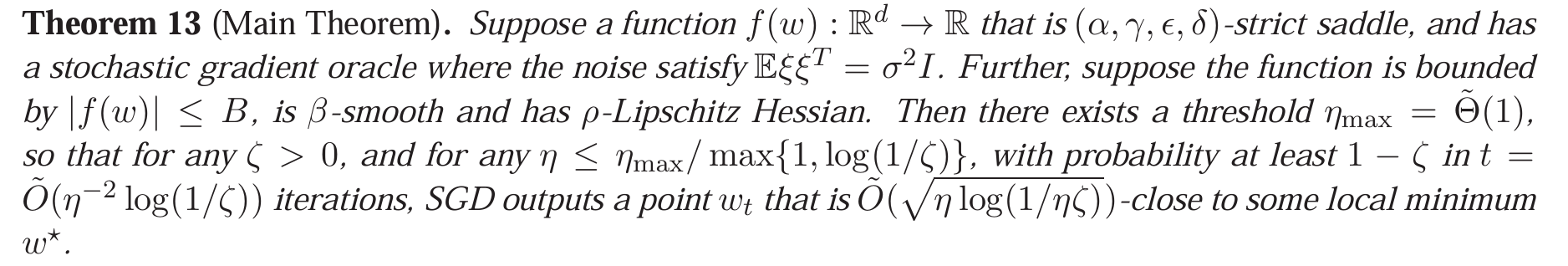
Theorem 18. For a bounded, smooth, Hessian smooth and strict saddle function $f$, SGD converges to some local minimum at rate $\tilde\O(\sqrt[4]T)$ w.h.p. More specifically:
- Noise $\xi$ must satisfy $\Ex(\xi^\top\xi)=\sigma^2I$.
- Hessian smooth means Lipschitz condition on $\nabla^2f$.
- $f$ needs to satisfy: if at some point $x$, $|\nabla f(x)|$ is small, $\lambda_{\min}(\nabla^2f(x))$ is not large negative, then there must be a local minimum near $x$ and $f$ must be strongly convex near $x$. This condition can be further specified by four parameters, whose polynomial determines the constant inside the convergence rate.
- The rate also depends on $\log\zeta^{-1}$ if we want to achieve $1-\zeta$ probability.
Proof strategy.
- When $|\nabla f|$ is large, we can use the methods already taught to show that each step the value of $f$ must decrease by some constant.
- When close to a local minimum, use martingale-related theory (Azuma’s inequality) to show that the probability of leaving the local-minimum neighborhood within a certain number of steps is small.
- When $|\nabla f|$ is small but the point is a saddle point/local maximum rather than a local minimum, use the existence of a negative direction in $\nabla^2 f$ to show that SGD’s random perturbation makes $x$ find that negative direction and escape the saddle point (note that if it finds a positive direction, it quickly returns). Specifically, if $\lambda_{\min}(\nabla^2 f(x))\le-\gamma$, first assume the neighborhood of $x$ is a perfect quadratic surface (dropping higher-order terms in the Taylor expansion), and use a similar taught method to show escape is guaranteed (the value of $f$ decreases by some constant after several steps). Then use martingale theory to show that the actual trajectory is close to the ideal trajectory with high probability.
- For the first and third cases, since $f$ is bounded above and below, they cannot happen too many times; therefore, within a certain number of steps, with high probability there is at least one moment near a local minimum, after which we use the second case.
Generalization Theory
Settings & Notes on Type-safe Requirements
There are several objects under the setting of generalization theory:
- Domain of input data $X$
- Labeling function $f:X\to\set{0,1}$
- Probability distribution on data $\pd\in\Delta(X)$
- Joint distribution on data and label $\pd\in\Delta(X\times\set{0,1})$
- Training input $S\in X^m$
- Training data $S\in\set{(x,f(x))\mid x\in X}^m$
- Hypothesis $h:X\to\set{0,1}$
- Hypothesis class $\hy\subseteq\set{h:X\to\set{0,1}}$
- Learning algorithm $A:(X\times\set{0,1})^{*}\to(X\to\set{0,1})$
- Loss function of some distribution and label function $L_{\pd,f}(h)=\Ex_{x\sim\pd}[h(x)\ne f(x)]$
- Loss function of some joint distribution $L_{\pd}=\Ex_{(x,y)\sim\pd}[h(x)\ne y]$
- Loss function of some inputs and label function $L_{S,f}=\sum_{x\in S}[h(x)\ne f(x)]/|S|$
- This collection of objects can certainly be characterized well in the language of category theory; maybe I’ll add it later.
The most annoying thing is that the learning algorithm only receives a sequence/set of pairs (labeled data), but this forces us to either use the joint distribution (which needs a stupid realizability claim), or project $S$ to the sequence/set consisting only of inputs, $S|x$, thus complicating the notation. So below, I will treat $S$ ambiguously: it includes labels only when plugged into $A$ or sampled from the joint distribution (in the agnostic PAC case), and at other times it only contains inputs.
Binary Classification
Theorem 1 (no-free-lunch). $\forall$ learning algorithm $A$ for binary classification, $\forall m\le |X|/2$, $\exists\pd\in\Delta(X),f:X\to\set{0,1}$, $$ \Pr_{S\sim\pd^m}\left[L_{\pd,f}(A(S))\ge\frac18\right]\ge\frac17 $$ Proof. If we can prove $$ \exists\pd,f,\Ex_{S\sim\pd^m}\left(L_{\pd,f}(A(S))\right)\ge\frac14\tag{1} $$ then by an argument similar to the proof of Markov inequality, $$ \eq{ &1\times\Pr_{S\sim\pd^m}\left[L_{\pd,f}(A(S))\ge\frac18\right]+\frac18\times\Pr_{S\sim\pd^m}\left[L_{\pd,f}(A(S))\le\frac18\right]\ge\Ex_{S\sim\pd^m}\left(L_{\pd,f}(A(S))\right)\ge\frac14\\ \implies{}&\frac78\times\Pr_{S\sim\pd^m}\left[L_{\pd,f}(A(S))\ge\frac18\right]+\frac18\ge\frac14\\ \implies{}&\Pr_{S\sim\pd^m}\left[L_{\pd,f}(A(S))\ge\frac18\right]\ge\frac17 } $$ So now let’s prove $(1)$. For simplicity assume $|X|=2m$. Just let $$ \pd(x)=\frac{1}{2m},\forall x\in X $$ There are $2^{2m}$ different $f$. $$ \eq{ &\frac1{2^{2m}}\sum_f\Ex_{S\sim\pd^m}(L_{\pd,f}(A(S)))\\ ={}&\frac1{2^{2m}}\sum_f\frac{1}{(2m)^m}\sum_SL_{\pd,f}(A(S))\\ \ge{}&\frac1{2^{2m}}\sum_f\frac{1}{(2m)^m}\sum_S\frac1{2m}\sum_{x\notin S}[A(S)(x)\ne f(x)]\\ ={}&\frac{1}{(2m)^m}\sum_S\frac1{2^{2m}}\frac1{2m}\sum_{f_0,f_1}\left(\sum_{x\notin S}[A(S)(x)\ne f_0(x)]+\sum_{x\notin S}[A(S)(x)\ne f_1(x)]\right)\\ \ge{}&\frac{1}{(2m)^m}\sum_S\frac{1}{2^{2m}}\frac1{2m}2^{2m-1}m\\ ={}&\frac14 } $$
Here the key step is that we pair every two labeling functions, so that they behave the same on $S$ and behave the opposite on $X\setminus S$. Like this: $$ \begin{matrix} x:&\square&\triangle&\diamonds&\hearts&\spades&\bigstar&\clubs&\maltese\\ \hline f_0:&\color{green}0&\color{green}1&\color{green}1&\color{green}0&\color{red}0&\color{green}1&\color{green}0&\color{red}1\\ f_1:&\color{green}0&\color{green}1&\color{green}1&\color{green}0&\color{green}1&\color{red}0&\color{red}1&\color{green}0\\ A(\set{\square,\triangle,\diamonds,\hearts}):&0&1&1&0&1&1&0&0 \end{matrix} $$
- This theorem does not mention the hypothesis class, but clearly here $\hy$ is the full set.
Definition 1. W.r.t. some $\hy,\pd,f$, the realizability assumption means $\exists h\in\hy$ achieving zero loss on $L_{\pd,f}$. The Empirical Risk Minimization (ERM) hypothesis class on training set $S$ is $\ERM_{\hy}(S)=\argmin_{h\in\hy}L_{S,f}(h)\subseteq\hy$.
- There are two cases where the realizability assumption fails: one is that $f$ is random, i.e., the label is not fixed for the same data point; the other is that $\hy$ does not cover all $2^{|X|}$ possibilities.
- Now we have four types of hypotheses from best to worst: the Bayes optimal predictor (which knows, for each data point, the probabilities of the two labels and outputs the more probable one), $\argmin_{h\in\hy}L_{\pd}(h)$, ERM, and an arbitrary hypothesis. For $h\in\hy$, we can decompose its loss as $L_{\pd}(h)=\epsilon_{\rm app}+\epsilon_{\rm est}$, where:
- $\epsilon_{\rm app}=\min_{h\in\hy}L_{\pd}(h)$ is the approximation error, representing the best achievable loss within the current hypothesis class. To optimize it, we need to enlarge $\hy$, but no matter how much we enlarge it, there is a lower bound: $L_\pd(\text{Bayes optimal predictor})$.
- $\epsilon_{\rm est}=L_{\pd}(h)-\epsilon_{\rm app}$ is the estimation error. For hypotheses trained from training data, it measures the distortion caused by minimizing empirical loss (the gap to population loss). To optimize it, we need to increase $m$.
Theorem 2. For finite $\hy$ and $\delta,\eps\in(0,1)$, let $m\ge\frac{\log(|\hy|/\delta)}{\eps}$. $\forall\pd,f$ for which the realizability assumption holds, $$ \Pr_{S\sim\pd^m}\left[\forall h\in\ERM_{\hy}(S),L_{\pd,f}(h)\le\eps\right]\ge 1-\delta $$ Proof. $$ \eq{ &\Pr_{S\sim\pd^m}\left[\exists h\in\ERM_{\hy}(S),L_{\pd,f}(h)>\eps\right]\\ \le{}&\sum_{h\in \hy\mid L_{\pd,f}(h)>\eps}\Pr_{S\sim\pd^m}[L_{S,f}(h)=0]&[\text{union bound}]\\ ={}&\sum_{h\in \hy\mid L_{\pd,f}(h)>\eps}\prod_{i=1}^m\Pr_{x_i\sim\pd}[h(x_i)=f(x_i)]&[\text{independency}]\\ \le{}&\sum_{h\in \hy\mid L_{\pd,f}(h)>\eps}(1-\eps)^m\\ \le{}&|\hy|(1-\eps)^m\\ \le{}&|\hy|\e^{-\eps m}\\ \le{}&\delta } $$
- Intuitively, failure to learn can happen when representation power is too strong: after fitting the given data, predictions on unseen data can still be arbitrary. Learning succeeds when representation power is not too strong: even if you union-bound all hypotheses that perform well on training data but poorly in reality, the total probability remains small. The key point here is $|\hy|$.
Definition 2. An $\hy$ is PAC learnable, iff $\exists m_{\hy}:(\eps,\delta)\mapsto m$ and a learning algorithm $A$, s.t. $\forall \pd\in\Delta(X),f$ that satisfies the realizability assumption, $$ \Pr_{S\sim\pd^{\ge m}}\left[L_{\pd,f}(A(S))\le\eps\right]\ge 1-\delta $$ Note that the hypothesis that $A$ returns is not necessarily ERM.
Corollary. Finite hypothesis class is PAC learnable.
Definition 3. An $\hy$ is agnostic PAC learnable, iff $\exists m_{\hy}:(\eps,\delta)\mapsto m$ and a learning algorithm $A$, s.t. $\forall \pd\in\Delta(X\times\set{0,1})$, $$ \Pr_{S\sim\pd^{\ge m}}\left[L_{\pd}(A(S))\le\min_{h\in\hy}L_{\pd}(h)+\eps\right]\ge 1-\delta $$ Obviously agnostic PAC learnable is stronger than (implies) PAC learnable. Surprisingly under (binary) classification settings, PAC learnable $\implies$ agnostic PAC learnable, but the proof is nontrivial.
Theorem 3. Some infinite hypothesis classes are also PAC learnable, for example $\hy=\set{h_a(x)=[x<a]\mid a\in\R\cup\set{\pm\infty}}$.
Proof strategy. Let $$ m_{\hy}(\eps,\delta)=\frac{\lceil\log\delta^{-1}\rceil}{\eps} $$ and $$ A(S)=h_a\text{ where }a=\max_{x\in S\mid f(x)=1}x $$ If the learned $a$ is within a neighborhood of $a_{*}$ whose probability mass is $\le\eps$, then we are good. The probability of the converse is $(1-\eps)^m\le\delta$.
- In class, someone asked whether a discrete distribution $\pd$ causes issues. If we use the above $A$ directly, it indeed can cause problems, e.g., $\pd(x)=\delta(x)$. The key detail is that the hypothesis is $[x<a]$; if we change it to $[x\le a]$, there is no issue. If it must be $[x<a]$, we can proceed in another way, namely by finding the smallest point whose label is $0$.
Definition 4. An $\hy$ shatters some finite set $C\subseteq X$, iff for each of the label combination in $\set{0,1}^{|C|}$, there exists a hypothesis in $\hy$ output it on $C$. The Vapnik–Chervonenkis (VC)-dimension of some $\hy$ is the maximal size of $C$ shattered by it. Specifically, if $\hy$ can shatter sets of arbitrary large size, then it has infinite VC-dimension.
Theorem 4 (generalized no-free-lunch). If some $\hy$ shatters some set of size $2m$, then $\forall A$, $\exists\pd$, $\exists h\in\hy$ (acts as realizability assumption), $$ \Pr_{S\sim\pd^{\le m}}\left[L_{\pd,f}(A(S))\ge\frac18\right]\ge\frac17 $$ Corollary. Infinite VC-dimension hypothesis class is not PAC learnable.
Theorem 5 (the fundamental theorem of statistical learning). For some $\hy$, $$ \VC(\hy)<\infty\iff\hy\text{ is PAC learnable}\iff\hy\text{ is agnostic PAC learnable}\iff\text{any ERM is a successful (agnostic) PAC learner} $$ Quantitatively, $\forall\hy$ such that $\VC(\hy)=d<\infty$, $\hy$ is agnostic PAC learnable with $$ m_{\hy}(\eps,\delta)=\Theta\left(\frac{d+\log\delta^{-1}}{\eps^2}\right) $$ and $\hy$ is PAC learnable with $$ \Omega\left(\frac{d+\log\delta^{-1}}{\eps}\right)\le m_{\hy}(\eps,\delta)\le\Omicron\left(\frac{d\log\eps^{-1}+\log\delta^{-1}}{\eps}\right) $$ Note that the lower bound indicates that there exist some $\pd$ and $f$ causing the learning algorithm to fail when the size of training data is below some constant $C$ times the quantity.
The proof involves Rademacher complexity, so here I only mention the intuition for the bound in the agnostic case. The strategy is to estimate the error rate of every hypothesis using $m$ samples. The requirement is that we should not mix up the best hypothesis with bad hypotheses that have population losses $>\min L+\eps$; in other words, the estimation error should be $\le\eps/2$ w.h.p. So we can use the Chernoff bound (where $\eps^2$ appears) and then the union bound.
Regression
TBD
Supervised Learning
Here I skip the part about settings.
Perceptron
Definition 1. For a binary classification problem, perceptron is simply $f_w(x)=\sgn(w^\top x)$. There’s a learning algorithm for perceptron: when it misclassifies at least one data point, randomly pick some input $x$ on which it fails, $w\xleftarrow{+}y\cdot x$, so that $w^\top x$ moves one step toward the correct sign.
Theorem 1. When the data is linearly separable, moreover, $\exists$ unit vector $w_{*}$ and $\gamma>0$ s.t. $\forall i$, $y_i(w_{*}^\top x_i)\ge\gamma$ (i.e. there’s a $2\gamma$ gap), if all $\|x_i\|\le R$, then the perceptron learning algorithm converges in $\O(\frac{R^2}{\gamma^2})$ steps.
Proof. For simplicity we assume $w_0=0$. On one hand $$ \eq{ \ip{w_t,w_{*}}&=\ip{w_{t-1}+y_{t-1}x_{t-1},w_{*}}\\ &=\ip{w_{t-1},w_{*}}+y_{t-1}(w_{*}^\top x_{t-1})\\ &\ge\ip{w_{t-1},w_{*}}+\gamma\\ &\ge \gamma t } $$ On the other hand $$ \eq{ \|w_t\|^2&=\|w_{t-1}\|^2+2y_{t-1}\ip{w_{t-1},x_{t-1}}+\|x_{t-1}\|^2\\ &\le\|w_{t-1}\|^2+\|x_{t-1}\|^2\\ &\le\|w_{t-1}\|^2+R^2\\ &\le R^2t } $$ So $$ \gamma^2t^2\le\ip{w_t,w_{*}}^2\le\|w_t\|^2\le R^2t\implies t\le\frac{R^2}{\gamma^2} $$
Linear Regression
Definition 2 (Kullback–Leibler divergence). $$ \mathrm{KL}(p\parallel q)=H(p,q)-H(p)=\int p(x)\log\frac{p(x)}{q(x)}\d x $$ Note that this is not a metric since it’s asymmetric and violates triangle inequality.
- Note the order. There are two intuitive views: first, the extra bits needed to encode $p$ using the optimal code for $q$; second, the “surprisal” when $p$ is treated as the reference distribution while the actual distribution is $q$. One clear point is that KL divergence penalizes cases where $p(x)\ne 0$ but $q(x)\approx 0$.
Definition 3. For linear regression problem $f(x)=w^\top x$, ridge regression comes from the motivation of minimizing $L(f,X,Y)$ while restricting $\|w\|_2^2\le c$, and its actual form is $\min. L(f,X,Y)+\frac\lambda2\|w\|_2^2$.
Definition 4. If we want to minimize $L(f,X,Y)$ while restricting $\|w\|_0\le c$, then the problem is non-differentiable. $\|w\|_1$ can approximate $\|w\|_0$, so we finally turn the goal to $\min. L(f,X,Y)+\lambda\|w\|_1$. Furthermore, regular GD cannot be used because when some parameter is between $\pm\eta\lambda$ it will never converge. So in practice we should use a proximal step, that is $$ w_{t+1}=\sgn(w_t-\eta\nabla L)\odot\max(|w_t-\eta\nabla L|-\eta\lambda,0) $$ and it’s called LASSO regression. The name is from “least absolute shrinkage and selection operator”.
Compressed Sensing
Theorem 2 (Nyquist). $2f_0$ sampling rate is needed to fully reconstruct a signal with no frequency higher than $f_0$.
Proof strategy. Let $y(x)$ and $Y(x)$ be the original function and the function after Fourier transform. The sampling function is $$ \text{Ш}_{1/f}(x)=\sum_n\delta(x-n/f) $$ and its Fourier transform can be proven to be $$ \fF[\text{Ш}_{1/f}](x)=f\text{Ш}_f(x)=f\sum_n\delta(x-fn) $$ Since the Fourier transform of a Hadamard product is the convolution of the two Fourier transforms, in frequency space, $\text{Ш}_{1/f}\cdot y$ will be the summation of $Y$ shifted by $0$, $\pm f_0$, $\pm 2f_0$, etc. In order to make these replicates not overlap causing aliasing, we need $f\ge 2f_0$.
Definition 5. However, real-world signals are usually sparse. For a vector $x\in\R^d$ that is sparse (low $\|x\|_0$), define the observation vector $y=Ax\in\R^n$ where $n\ll d$ and $A$ is a fat matrix called the measurement matrix. Given only $y$ and $A$, it is usually possible to recover $x$ (uniquely, with the least number of nonzero entries). Thus a high-dimensional sparse vector is compressed into a low-dimensional vector, which is called compressed sensing.
- A real-world example is that $A$ is obtained by multiplying a measurement matrix $M$ and a basis matrix $\Psi$. For face images, $\Psi$ is the set of eigenfaces, $x$ is the weight of each eigenface, $\Psi x$ is the observed image, and $A\Psi x$ is some compressed result. For signals, $x$ is frequency information, $\Psi$ is a basis of waves at different frequencies, and $M$ is the sampling matrix.
So now the task is $$ \argmin_{x: Ax=y}\|x\|_0\longrightarrow\argmin_{x:Ax=y}\|x\|_1 $$ by Lagrange multiplier, the function to be minimized becomes $$ \|x\|_1-\lambda(Ax-y) $$ or equivalently, $$ \|x\|_1+\lambda\|Ax-y\|_2^2 $$ or we can imagine there is noise $y=Ax+\xi$, then without Lagrange multiplier the goal is $\min.\eta\|y-Ax\|_2^2+\|x\|_0$. Either of these conversions leads to exactly the same form as LASSO regression, differing only in meaning.
| meanings | $y$ | $A$ | $x$ | $\lambda$ |
|---|---|---|---|---|
| CS | observation | measurement | signal | multiplier/coef on noise |
| LASSO | output | input | weights | regularization |
Definition 6. A matrix $W\in\R^{n\times d}$ is $(\epsilon,s)$-RIP (restricted isometry property), iff $\forall x\in\R^d$ s.t. $\|x\|_0\le s$, $(1-\epsilon)\|x\|_2^2\le\|Wx\|_2^2\le(1+\epsilon)\|x\|_2^2$.
Theorem 3. Let $W$ be a $(\epsilon,2s)$-RIP matrix with $\epsilon<1$, then $\forall x$ with $\|x\|_0\le s$, $$ \argmin_{v:Wv=Wx}\|v\|_0=\set{x} $$ Proof. If there’s $v\ne x$ such that $Wv=Wx$ and $\|v\|_0\le\|x\|_0$ then $W(v-x)=0$, violating $(1-\epsilon)\|x-v\|_2^2\le\|W(x-v)\|_2^2$.
Theorem 4. Let $W$ be a $(\epsilon,2s)$-RIP matrix with $\epsilon<\frac1{1+\sqrt2}$, then $\forall x$ with $\|x\|_0\le s$, $$ \argmin_{v:Wv=Wx}\|v\|_1=\set{x} $$ Proof. In theorem 5, $x=x_s$.
Theorem 5. Let $W$ be a $(\epsilon,2s)$-RIP matrix with $\epsilon<\frac1{1+\sqrt2}$, then $\forall x$, let $x_s$ be any vector preserving the $s$ largest (in absolute value) elements of $x$ and other elements being $0$, then $$ \forall \tilde x\in\argmin_{v:Wv=Wx}\|v\|_1, \|\tilde x-x\|_2\le\frac{2(1+\rho)s^{-1/2}}{1-\rho}\|x-x_s\|_1\text{ where }\rho=\frac{\sqrt2\epsilon}{1-\epsilon} $$
Note that if $\epsilon=\frac{1}{1+\sqrt2}$, $\rho=1$.
Proof. Denote $(x_I)_i=[i\in I]x_i$. Let $h=\tilde x-x$.
Partition the indices $[d]$ into $d/s$ sets $T_0\sim T_{d/s-1}$. $T_0=\text{top-}s\argmax_{i\in[d]}|x_i|$, and for $i\ge 1$, $$ T_k=\text{top-}s\argmax_{i\in[d]\setminus\bigcup_{j=0}^{k-1}T_j}|h_i| $$ So we need to bound $\|h\|_2$ by $\|x_{\overline{T_0}}\|_1$.
Consider $T_0\cup T_1$ ($T_{0,1}$ in short); it contains indices of large elements in $x$ and $\tilde x$. The idea is, $$ \|h\|_2\le\|h_{T_{0,1}}\|_2+\|h_{\overline{T_{0,1}}}\|_2 $$ and we bound these two components respectively.
$$ \eq{ \|h_{\overline{T_{0,1}}}\|_2&\le\sum_{k\ge 2}\|h_{T_k}\|_2\\ &\le\sum_{k\ge 2}s^{1/2}\|h_{T_k}\|_{\infty}\\ &\le\sum_{k\ge 2}s^{-1/2}\|h_{T_{k-1}}\|_1\\ &\le\sum_{k\ge 1}s^{-1/2}\|h_{T_k}\|_1\\ &=s^{-1/2}\|h_{\overline{T_0}}\|_1 } $$ Lemma 1. For disjoint $I,J\subset[d]$ with size $\le s$, $\lvert\ip{Wv_I,Wv_J}\rvert\le\epsilon\|v_I\|_2\|v_J\|_2$.
Proof. $$ \eq{ \ip{Wv_I,Wv_J}&=\frac{\|W(v_I+v_J)\|_2^2-\|W(v_I-v_J)\|_2^2}{4}\\ &\le\frac{(1+\epsilon)\|v_I+v_J\|_2^2-(1-\epsilon)\|v_I-v_J\|_2^2}{4}\\ &=\frac{\epsilon}{2}\left(\|v_I\|_2^2+\|v_J\|_2^2\right)\\ \implies\ip{W\hat v_I,W\hat v_J}&\le\epsilon\\ \implies\ip{W v_I,W v_J}&\le\epsilon\|v_I\|_2\|v_J\|_2 } $$ Similarly $\ip{W v_I,W v_J}\ge-\epsilon\|v_I\|_2\|v_J\|_2$. $$ \eq{ (1-\epsilon)\|h_{T_{0,1}}\|_2^2&\le\|Wh_{T_{0,1}}\|_2^2\\ &=\ip{Wh_{T_0}+Wh_{T_1},-Wh_{T_2}-Wh_{T_3}-\cdots}\\ &\le\epsilon\left(\|h_{T_0}\|_2+\|h_{T_1}\|_2\right)\sum_{k\ge 2}\|h_{T_k}\|_2\\ &\le\sqrt2\epsilon\|h_{T_{0,1}}\|_2\sum_{k\ge 2}\|h_{T_k}\|_2\\ &\le\sqrt2\epsilon\|h_{T_{0,1}}\|_2s^{-1/2}\|h_{\overline{T_0}}\|_1\\ \implies\|h_{T_{0,1}}\|_2&\le\frac{\sqrt2\epsilon}{1-\epsilon}s^{-1/2}\|h_{\overline{T_0}}\|_1 } $$ Now $$ \left\{ \eq{ \|h_{T_{0,1}}\|_2&\le\rho s^{-1/2}\|h_{\overline{T_0}}\|_1\\ \|h_{\overline{T_{0,1}}}\|_2&\le s^{-1/2}\|h_{\overline{T_0}}\|_1 } \right. $$ Lemma 2. $\|h_{\overline{T_0}}\|_1\le\|h_{T_0}\|_1+2\|x_{\overline{T_0}}\|_1$.
Proof. $$ \left\{ \eq{ \|x+h\|_1&\le\|x\|_1\\ \|x\|_1&=\|x_{T_0}\|_1+\|x_{\overline{T_0}}\|_1\\ \|x+h\|_1&=\|(x+h)_{T_0}\|_1+\|(x+h)_{\overline{T_0}}\|_1\ge\|x_{T_0}\|_1-\|h_{T_0}\|_1+\|h_{\overline{T_0}}\|_1-\|x_{\overline{T_0}}\|_1 } \right. $$ Substitute then shift the terms. Here is the visual intuition:
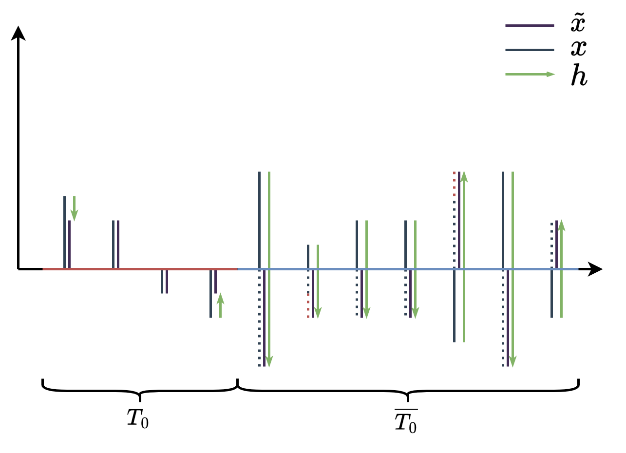
Furthermore, we have $$ s^{-1/2}\|h_{\overline{T_0}}\|_1\le s^{-1/2}\|h_{T_0}\|_1+2s^{-1/2}\|x_{\overline{T_0}}\|_1\le\|h_{T_0}\|_2+2s^{-1/2}\|x_{\overline{T_0}}\|_1 $$ Now $$ \eq{ \|h_{T_{0,1}}\|_2&\le\rho s^{-1/2}\|h_{\overline{T_0}}\|_1\\ &\le\rho\left(\|h_{T_0}\|_2+2s^{-1/2}\|x_{\overline{T_0}}\|_1\right)\\ &\le\rho\|h_{T_{0,1}}\|_2+2\rho s^{-1/2}\|x_{\overline{T_0}}\|_1\\ \implies\|h_{T_{0,1}}\|_2&\le\frac{2\rho}{1-\rho}s^{-1/2}\|x_{\overline{T_0}}\|_1 } $$ and $$ \eq{ \|h_{\overline{T_{0,1}}}\|_2&\le s^{-1/2}\|h_{\overline{T_0}}\|_1\\ &\le\|h_{T_{0,1}}\|_2+2s^{-1/2}\|x_{\overline{T_0}}\|_1\\ &\le\frac{2}{1-\rho}s^{-1/2}\|x_{\overline{T_0}}\|_1 } $$ So $$ \|h\|_2\le\|h_{T_{0,1}}\|_2+\|h_{\overline{T_{0,1}}}\|_2\le\frac{2(1+\rho)}{1-\rho}s^{-1/2}\|x_{\overline{T_0}}\|_1 $$
Theorem 6. For some $d$, $s$, for some $n=\Theta(\epsilon^{-2}s\log(d/\delta\epsilon))$, let $W\in\R^{n\times d}$ where i.i.d. $W_{i,j}\sim\Nd(0,1/n)$. w.p. $\ge 1-\delta$, $W$ is $(\epsilon,s)$-RIP.
The norms taken below are all $\ell_2$-norm.
Lemma. $\exists Q\subset\R^d$ of $\O(\epsilon^{-1})^d$ points, s.t. $\forall\|x\|\le 1$, $\min_{v\in Q}\|x-v\|\le\epsilon$.
Proof. Construct $$ Q_0=\Set{-1,\frac{1-k}k,\cdots,0,\frac1k,\cdots,1}^d\cap \overline B_d(1) $$ so that $$ \min_{v\in Q}\|x-v\|\le\sqrt{\left(\frac1{2k}\right)^2\cdot d}=\frac{\sqrt d}{2k} $$ We can take $k\ge\sqrt d/2\epsilon$. To estimate $|Q_0|$, we associate each point $x$ with the cube $x+[-1/2k,+1/2k]^d$. This implies that $\overline B_d(1+\sqrt d/2k)$ must contain all the cubes, so we can comfortably approximate $|Q_0|$ by the following method, without asymptotical error: $$ \eq{ |Q_0|&\approx\frac{V_d}{(1/k)^d}\\ &=\frac{\pi^{d/2}}{\Gamma(d/2+1)}k^d\\ &\approx\frac{\pi^{d/2}\e^{d/2+1}}{\sqrt{2\pi}(d/2+1)^{d/2-1}}\frac{d^{d/2}}{2^d\epsilon^d}\\ &\approx\left(\sqrt{\frac{\pi\e}2}\epsilon^{-1}\right)^d=\O(\epsilon^{-1})^d } $$ Lemma (Johnson–Lindenstrauss). $\forall Q\subset\R^d$, for some $n=\Theta(\epsilon^{-2}\log(|Q|/\delta))$, let $W\in\R^{n\times d}$ where i.i.d. $W_{i,j}\sim\Nd(0,1/n)$, w.p. $\ge 1-\delta$, $\forall x\in Q$, $(1-\epsilon)\|x\|^2\le\|Wx\|^2\le(1+\epsilon)\|x\|^2$.
Proof. For the complete proof of JL lemma, refer to this post. I’d like to review the proof sketch here.
We can normalize $x\in Q$. Let $w_i$ be the $i$-th row of $W$, then $w_ix\sim\Nd(0,1/n)$ and $\|Wx\|^2\sim\chi_n^2/n$. By some tail bound, $$ \Pr[\|Wx\|^2\notin[1-\epsilon,1+\epsilon]]\le\e^{-\Omega(n\epsilon^2)} $$ and can be simplified as $\delta/|Q|$. Then apply union bound.
Lemma. $\forall Q\subset\R^d$ of $s$ orthonormal vectors, for some $n=\Theta(\epsilon^{-2}(\log\delta^{-1}+s\log\epsilon^{-1}))$, let $W\in\R^{n\times d}$ where i.i.d. $W_{i,j}\sim\Nd(0,1/n)$, w.p. $\ge 1-\delta$, $\forall x\in\span Q$, $(1-\epsilon)\|x\|\le\|Wx\|\le(1+\epsilon)\|x\|$.
Proof. Let $U\in\R^{s\times|Q|}$ be the matrix consisting of vectors in $Q$ as column vectors. Apply JL lemma on $\set{Uv\mid v\in Q_0}$ where $Q_0$ is the set constructed in the proof of lemma 1. Here we need $n=\Theta(\epsilon^{-2}\log(\O(\epsilon^{-1})^s/\delta))=\Theta(\epsilon^{-2}(\log\delta^{-1}+s\log\epsilon^{-1}))$. The result of JL lemma also implies $(1-\epsilon)\|x\|\le\|Wx\|\le(1+\epsilon)\|x\|$.
Assume $\max_{\|x\|=1}\lVert Wx\rVert=1+a$. Consider any unit vector $x\in\span Q$, $x=Ux_0$. Then by lemma 1, $\exists v\in Q_0$ such that $$ \eq{ \|Wx\|&\le\|WUv\|+\|WU(x_0-v)\|\\ &\le(1+\epsilon)\|Uv\|+(1+a)\|U(x_0-v)\|\\ &=(1+\epsilon)\|v\|+(1+a)\|x_0-v\|\\ &\le1+\epsilon+(1+a)\epsilon\\ \implies1+a&\le1+\epsilon+(1+a)\epsilon\\ \implies a&\le\frac{2\epsilon}{1-\epsilon} } $$ and $$ \eq{ \|Wx\|&\ge\|WUv\|-\|WU(x_0-v)\|\\ &\ge(1-\epsilon)\|v\|-(1+a)\|x_0-v\|\\ &\ge(1-\epsilon)(\|x_0\|-\|x_0-v\|)-(1+a)\|x_0-v\|\\ &\ge1-\epsilon-(2-\epsilon+a)\epsilon\\ &\ge1-3\epsilon-\epsilon^2-\frac{2\epsilon^3}{1-\epsilon} } $$ Scale $\epsilon$ to get the final result.
Proof of the original theorem. Two more details to go.
- By $[(1-\epsilon)^2,(1+\epsilon)^2]\subset[1-3\epsilon,1+3\epsilon]$, restore the square.
- Enumerate $Q$ over all $s$-element subsets of $\set{e_1,\cdots,e_d}$, and apply union bound. Now the probability becomes $1-\binom ds\delta$ so we should shrink $\delta$ by $\binom ds$ for every individual $Q$. The final $n$ will be $\Theta(\epsilon^{-2}\log(\binom ds\delta^{-1})+s\log\epsilon^{-1})\le\Theta(\epsilon^{-2}s\log(d/\delta\epsilon))$.
This theorem actually addresses the question of why compressed sensing can be used in real-life scenarios. If $v$ is some data that is not sparse but possesses some implicit sparsity, that is, $v=Ux$ for some orthonormal matrix $U$ and sparse vector $x$, then applying measurement to $v$ using some Gaussian matrix $W$ is also applying that to $x$ because $WU$ is also Gaussian. One can easily check that by calculating the variance and covariance. So the main point now becomes finding a set of “features”.
If $v$ is obtained by applying some nonlinear transformation $G(\cdot)$ on $x$, there are also such kinds of guarantees:
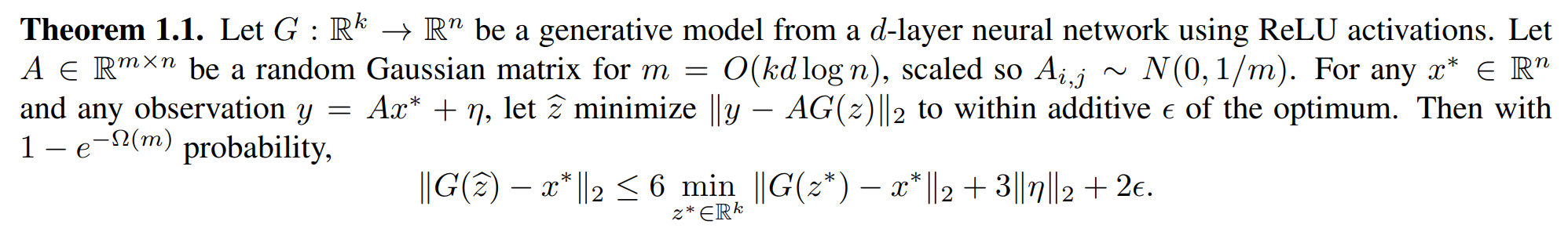
Support Vector Machine
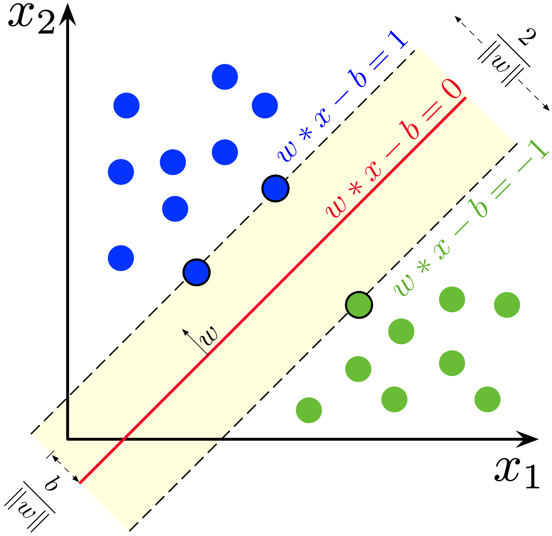
Definition 7. For a linear classification problem, a support vector machine (SVM) constructs a linear separator, the one with the largest margin. Margin is defined as the distance from the separator to the closest point. Let the classifier be $f(x)=w^\top x-b$. If there’s a point $x_+$ labeled $+$, then $f(x_+)$ should be $>0$ and by geometry, the margin is $\frac{|w^\top x_+-b|}{\|w\|_2}$. In other words, the problem becomes $$ \max.\frac{1}{\|w\|_2}\quad\text{s.t. }y_i(w^\top x_i-b)\ge 1 $$
If the data is not linearly separable, a penalty term is added, converting it to a relaxed version $$ \min.\|w\|_2+\lambda\sum_i[y_i(w^\top x_i-b)<1] $$ which is NP-Hard. A soft version is using hinge loss: $$ \min.\|w\|_2+\lambda\sum_i\max\set{1-y_i(w^\top x_i-b),0} $$ or $$ \min.\|w\|_2+\lambda\sum_i\xi_i\quad\text{s.t. } y_i(w^\top x_i-b)\ge 1-\xi_i,\;\xi_i\ge 0 $$ If we regard it as an L2 regularization, it’d better be $$ \min.\frac{\|w\|_2^2}2+\lambda\sum_i\xi_i\quad\text{s.t. } y_i(w^\top x_i-b)\ge 1-\xi_i,\;\xi_i\ge 0 $$
By convention, below I’ll write $w^\top x+b$ instead of $w^\top x-b$.
Theorem 7. For some optimization problem $$ \min. f(x)\quad\text{s.t. }g_i(x)\le 0,\;h_j(x)=0 $$ Denote the optimal value as $p^{*}$.
Consider the Lagrangian $$ \la(x,\lambda,\nu)=f(x)+\sum_i\lambda_ig_i(x)+\sum_j\nu_jh_j(x) $$ There’s weak duality $$ \max_{\lambda\ge 0,\nu}\min_x\la(x,\lambda,\nu)\le p^{*} $$ Under some condition, the inequality can turn into equality, introducing strong duality. When the primal problem is convex (both objective function $f$ and the feasible set are convex) and differentiable, satisfies Slater’s condition, and has strong duality, $$ x^{*} \text{ is optimal}\iff\exists \lambda^{*},\nu^{*}\text{ satisfying KKT}. $$ where the KKT conditions are $$ \left\{\eq{ &g_i(x^{*})\le 0,\;h_j(x^{*})\le 0&(\text{Primal feasibility})\\ &\lambda_i^{*}\ge 0&(\text{Dual feasibility})\\ &\lambda_i^{*}g_i(x^{*})=0&(\text{Complementary slackness})\\ &\nabla_x\la(x^{*},\lambda^{*},\nu^{*})=0&(\text{Stationarity}) }\right. $$ Definition 8. The Lagrangian dual of the above optimization problem is $$ \max.\left(\min_x\la(x,\lambda,\nu)\right)\quad\text{s.t. }\lambda\ge 0 $$ Theorem 8. The dual problem of SVM, can be simplified as $$ \max.\sum_i\alpha_i-\frac12\sum_i\sum_j\alpha_i\alpha_jy_iy_j\ip{x_i,x_j}\quad\text{s.t. }0\le\alpha_i(\le\lambda),\;\sum_i\alpha_iy_i=0 $$ Proof. First consider linearly separable case. Recall the program $$ \max.\frac{1}{\|w\|_2}\quad\text{s.t. }y_i(w^\top x_i+b)\ge 1 $$ equivalently, $$ \boxed{\min.\frac{\|w\|_2^2}{2}\quad\text{s.t. }1-y_i(w^\top x_i+b)\le 0} $$ Lagrangian $$ \la(w,b,\alpha)=\frac{\|w\|_2^2}{2}-\sum_i\alpha_i(y_i(w^\top x_i+b)-1) $$ Now use the KKT condition to simplify $\la$ to be maximized. Take the gradient $$ \nabla_w\la(w,b,\alpha)=w-\sum_i\alpha_iy_ix_i=0\implies w=\sum_i\alpha_iy_ix_i $$
$$ \p_b\la(w,b,\alpha)=-\sum_i\alpha_iy_i=0 $$
Substitute back, $$ \la(w_{*},b,\alpha)=\frac12\left\|\sum_i\alpha_iy_ix_i\right\|_2^2-\sum_i\alpha_iy_ix_i\left(\sum_j\alpha_jy_jx_j^\top\right)+\sum_i\alpha_i=\sum_i\alpha_i-\frac12\sum_i\sum_j\alpha_i\alpha_jy_iy_j\ip{x_i,x_j} $$ Now the relaxed soft version: $$ \boxed{\min.\frac{\|w\|_2^2}2+\lambda\sum_i\xi_i\quad\text{s.t. } y_i(w^\top x_i+b)\ge 1-\xi_i,\;\xi_i\ge 0} $$ Lagrangian $$ \la(w,b,\xi,\alpha,\kappa)=\frac{\|w\|_2^2}2+\lambda\sum_i\xi_i-\sum_i\alpha_i(y_i(w^\top x_i+b)-1+\xi_i)-\sum_i\kappa_i\xi_i $$
$\nabla_w$ part and $\p_b$ part are the same. $$ \nabla_\xi\la=\lambda1-\alpha-\kappa=0\implies\alpha_i+\kappa_i=\lambda $$ Thus $$ \eq{ \la(w_{*},b,\xi,\alpha,\kappa)&=\frac12\left\lVert\sum_i\alpha_iy_ix_i\right\rVert_2^2+\sum_i(\alpha_i+\kappa_i)\xi_i-\sum_i\alpha_iy_ix_i\left(\sum_j\alpha_jy_jx_j^\top\right)+\sum_i\alpha_i-\sum_i\alpha_i\xi_i-\sum_i\kappa_i\xi_i\\ &=\sum_i\alpha_i-\frac12\sum_i\sum_j\alpha_i\alpha_jy_iy_j\ip{x_i,x_j} } $$ which is the same as the separable case.
Moreover: interpretation of $\alpha_i$:
- $\alpha_i=0$: the corresponding point is outside the margin (or coincidentally, on the margin) and can be deleted without affecting the result.
- $0<\alpha_i<\lambda$: the corresponding point is on the margin, and is the “supporting point”.
- $\alpha_i=\lambda$: the corresponding point is inside the margin / on the hyperplane / wrongly classified (or coincidentally, on the margin).
To get $w$, calculate $\sum_i\alpha_iy_ix_i$. To get $b$, by complementary slackness condition, if there’s some $\alpha_i\in(0,\lambda)$, then $b-y_iw^\top x_i$. Otherwise it’s the degenerated case, for example: $(x_1,y_1)=(1,1)$, $(x_2,y_2)=(-1,-1)$, $\lambda=0.25$. The dual problem is $$ \max.\alpha_1+\alpha_2-\frac12(\alpha_1+\alpha_2)^2\quad\text{s.t. }0\le\alpha_1,\alpha_2\le0.25,\alpha_1-\alpha_2=0 $$ Obviously we should choose $\alpha_1=\alpha_2=0.25$, thus $w=0.5$, and $b$ can be arbitrarily within $[-0.5,0.5]$. This scenario corresponds to that the penalty is so small that the optimal solution would rather violate the $y_i(w^\top x_i+b)\ge 1$ constraint than making $\|w\|$ big.
Q: In principle, why do we ever consider the dual SVM?
A: There are two evident reasons. First, usually there are only a few supporting points, thus $\alpha$ is sparse; second, the kernel trick can only be applied to dual SVM.
Definition 9. Kernel trick is an extension of SVM in the scenario where input points are originally inseparable but can be transformed by some nonlinear function to some higher-dimensional space and separated (think of a disk region, $f(x,y)=(x,y,x^2+y^2)$). Here the transformation is called $\phi$. The codomain of $\phi$ may have too high a dimension to be stored explicitly. Kernel trick is about not writing out the transformation result explicitly, and only calculating $\ip{\phi(x_i),\phi(x_j)}$. Specifically,
- $\la$ only involves calculating such inner products.
- To classify inputted point $x$, we need to calculate $w^\top x=\sum_i\alpha_iy_i\ip{\phi(x_i),\phi(x)}$.
The point is that $\ip{\phi(x_i),\phi(x_j)}$ can usually be computed in a faster way than adding the products of each component together. Note that in the primal SVM, there’s no such benefit.
Example. $\phi(x_1,\cdots,x_d)=(1,\sqrt2x_1,\cdots,\sqrt2x_d,x_1^2,\cdots,x_d^2,\sqrt2x_1x_2,\cdots,\sqrt2x_{d-1}x_d)\in\R^{\O(d^2)}$. $$ \ip{\phi(x),\phi(y)}=1+2\sum_ix_iy_i+\sum_ix_i^2y_i^2+\sum_i\sum_jx_ix_jy_iy_j=(\ip{x,y}+1)^2 $$ Theorem 9 (Mercer). Any positive semidefinite kernel’s matrix can be realized as a Gram matrix.
Decision Tree
Definition 10. A decision tree is a decision support recursive partitioning structure that uses a tree-like model of decisions and their possible consequences (taken from Wikipedia).
Definition 11. The greedy method of constructing a decision tree is as follows: now there are $n$ datapoints, each containing some inputs (attributes) and an output (correct answer). Select one of the input fields as the separating variable, which has the minimal weighted Gini index, then recursively call the division algorithm. For all the datapoints with some specific value on the specific input field ($x_k=x$ for some $k,x$), let the output be $y_{t_1},\cdots,y_{t_n}$, then the Gini index / Gini impurity is defined as $$ 1-\sum_y\left(\frac{\#[y_{t_i}=y]}{n}\right)^2=1-\sum_y\Pr_i[y_i=y\mid x_{i,k}=x]^2 $$ and the weighted Gini index is the weighted average across all $x_i=j$, i.e. $$ \sum_x\frac{\#[x_k=x]}{N}\mathrm{Gini}_{k,x}=\sum_x\Pr_i[x_{i,k}=x]\left(1-\sum_y\Pr_i[y_i=y\mid x_{i,k}=x]^2\right) $$ So it’s like an empirical version of information entropy.
Definition 12. Bagging is sampling random datapoints and random features (with replacement) and run (weak) learner on the sampled data. Random forest is to learn multiple (decision tree) models by bagging, then average/take the majority over the models when doing prediction.
Decision tree can overfit arbitrarily, while random forest / boosting reduces overfitting (in some strongest sense) and is even comparable to DL methods nowadays in some specific tasks.
Definition 13. Boosting is an optimized way of combining weak classifiers. Different from the random forest, boosting considers building trees sequentially, dynamically adjusting the probability distribution on training data according to the previous performance. AdaBoost is an algorithm that specifies the weight adjusting strategy:
- $D_1$ is the uniform distribution over the datapoints.
- Every round, train on the $D_t$ using weak learner, to get the weak classifier $h_t$.
- Let $\epsilon_t$ be the empirical loss (on $D_t$) of $h_t$. Let $\alpha_t=\frac12\ln \frac{1-\epsilon_t}{\epsilon_t}$. $D_{t+1}(i)\propto D_t(i)\cdot\exp(-\alpha_ty_ih_t(x_i))$. This means that if the prediction of $h_t$ is correct on datapoint $i$, scale down the weight assigned on it, otherwise scale up the weight.
- The final classifier is $H_{\rm final}(x)=\sgn(\sum_t\alpha_th_t(x))$
Notice that here $\epsilon_t$ should be $<1/2$ so that $\alpha_t>0$, meaning that $h$ cannot be some random guess.
Theorem 10. Let $\gamma_t=\frac12-\epsilon_t$. $L({H_{\rm final}})\le\exp(-2\sum_t\gamma_t^2)$. Thus if $\forall t$, $\gamma_t\ge\gamma>0$, then $L(H_{\rm final})\le\exp(-2T\gamma^2)$.
Proof. Denote the normalization coefficient of $D_{t+1}$ as $Z_t$. Assume the algorithm runs for $T$ rounds.
First, unwrap the definition recurrence of $D_{T+1}$: $$ D_{T+1}(i)=\frac1m\frac{\exp\left(-\sum_{t=1}^T\alpha_ty_ih_t(x_i)\right)}{\prod_{t=1}^TZ_t} $$ Second, expand the definition of $L(H_{\rm final})$: $$ \eq{ L(H_{\rm final})&=\frac1m\sum_i[y_i\ne H_{\rm final}(x_i)]\\ &=\frac1m\sum_i\left[y_i\sum_t\alpha_th_t(x_i)\le 0\right]\\ &\le\frac1m\sum_i\exp\left(-y_i\sum_t\alpha_th_t(x_i)\right)\\ &=\sum_iD_{T+1}(i)\prod_tZ_t\\ &=\prod_tZ_t } $$ Finally, bound $Z_t$. Intuitively, since the loss is $<1/2$, $Z_t$ should be $<1$. $$ \eq{ Z_t&=\sum_iD_t(i)\exp(-\alpha_ty_ih_t(i))\\ &=\exp(-\alpha_t)\sum_{i:h_t(i)=y_i}D_t(i)+\exp(\alpha_t)\sum_{i:h_t(i)\ne y_i}D_t(i)\\ &=\exp(-\alpha_t)(1-\epsilon_t)+\exp(\alpha_t)\epsilon_t\\ &=\sqrt{\frac{\epsilon_t}{1-\epsilon_t}}(1-\epsilon_t)+\sqrt{\frac{1-\epsilon_t}{\epsilon_t}}\epsilon_t\\ &=2\sqrt{\epsilon_t(1-\epsilon_t)}\\ &=2\sqrt{\frac14-\gamma_t^2}\\ &=\sqrt{1-4\gamma_t^2}\\ &=1-\frac12(4\gamma_t^2)-\frac{1}{8(1-\xi)^{3/2}}(4\gamma_t^2)\\ &\le1-2\gamma_t^2\\ &\le\exp(-2\gamma_t^2) } $$ Definition 14. AdaBoost is adaptive, in the sense that there’s no need to know $\gamma$ in order to determine any hyperparameter of the algorithm, contrary to the GD family (need $L$, $\mu$, etc.).
Experiments have shown that AdaBoost does not suffer from overfitting, which can also be explained by the following two theorems.
Theorem 11. It implies low population loss when the obtained classifier fits the training data with a considerable margin. Formally, w.p. $1-\delta$ over training data $S\sim D^m$, $\forall f$ being convex combination of hypotheses, $$ \Pr_{(x,y)\sim D}[yf(x)\le0]=\Pr_{(x,y)\sim U(S)}[yf(x)\le\theta]+\O\left(\frac1{\sqrt m}\left(\frac{\log m\log|\hy|}{\theta^2}+\log\frac1\delta\right)^{1/2}\right) $$ Theorem 12. The margin of AdaBoost increases with the number of iterations. Formally, let $f(x)=\sum_t\alpha_th_t(x)/\sum_t\alpha_t$ (so $H_{\rm final}(x)=\sgn(f(x))$ still), $$ \Pr_{(x,y)\sim U(S)}[yf(x)\le\theta]\le2^T\prod_t\sqrt{\epsilon_t^{1-\theta}(1-\epsilon_t)^{1+\theta}} $$ When $\theta\le 2\gamma$, by monotonicity, $$ 2^T\prod_t\sqrt{\epsilon_t^{1-\theta}(1-\epsilon_t)^{1+\theta}}\le2^T\prod_t\sqrt{\left(\frac12-\gamma\right)^{1-\theta}\left(\frac12+\gamma\right)^{1+\theta}}=\left(\sqrt{(1-2\gamma)^{1-\theta}(1+2\gamma)^{1+\theta}}\right)^T $$ When $\theta<-\frac{\log(1+2\gamma)+\log(1-2\gamma)}{\log(1+2\gamma)-\log(1-2\gamma)}\impliedby\theta<\gamma$, the term $<1$. So intuitively, the margin is at least $\frac12-\epsilon$, which is how better is the weak learner than random guess.
Proof. It’s basically the same as the proof of theorem 10. $$ \eq{ \Pr_{(x,y)\sim U(S)}[yf(x)\le\theta]&=\frac1m\sum_i\left[y_i\sum_t\alpha_th_t(x_i)\le\theta\sum_t\alpha_t\right]\\ &\le\frac1m\sum_i\exp\left(-y_i\sum_t\alpha_th_t(x_i)+\theta\sum_t\alpha_t\right)\\ &=\exp\left(\theta\sum_t\alpha_t\right)\prod_tZ_t\\ &=\prod_t\sqrt{\left(\frac{1-\epsilon_t}{\epsilon_t}\right)^\theta}2^T\prod_t\sqrt{\epsilon_t(1-\epsilon_t)}\\ &=2^T\prod_t\sqrt{\epsilon_t^{1-\theta}(1-\epsilon_t)^{1+\theta}} } $$ The inequalities $\epsilon_t^{1-\theta}(1-\epsilon_t)^{1+\theta}\le\epsilon^{1-\theta}(1-\epsilon)^{1+\theta}$ and $\gamma\le-\frac{\log(1+2\gamma)+\log(1-2\gamma)}{\log(1+2\gamma)-\log(1-2\gamma)}$ can both be proven by taking derivative.
Definition 15. Coordinate descent is to minimize along the coordinate direction at each step. A coordinate selection rule is needed.
Definition 16. Gradient boosting is the generalization of AdaBoost, or we can regard it as a unification of boosting and the additive model. The setting is an online descent process. Informally, consider a function $f$ that does not fit the points $(x_1,y_1)\sim(x_n,y_n)$ very well. It is straightforward to think that we should try to fit $(x_1,y_1-f(x_1)),\cdots,(x_n,y_n-f(y_n))$ using another model $h$ and let $f^\prime=f+h$. If $h$ is weak, we may iteratively find $h$ and add it to $f$.
Here comes the point. Such a process is a special case under a more general framework. For now regard $f$ as a variable. The goal is to minimize $L(f,X,Y)=\sum_i\ell(f,x_i,y_i)$. By GD, we expect $f^\prime=f-\eta\frac{\p L}{\p f}$; more concretely, $h(x_i)\approx\frac{\p\ell(y_i,f(x_i))}{\p f(x_i)}$ and $f^\prime=f-\eta h$. So the idea previously mentioned is just $\ell(y,\hat y)=(y-\hat y)^2/2$. For general gradient boosting, $\eta$ is chosen adaptively (this is natural since the partial derivative is a local property) so that $L(f^\prime,X,Y)$ is minimized.
Theorem 13. AdaBoost is the case of (discrete version of) gradient boosting under $\ell(y,\hat y)=\e^{-y\hat y}$.
Proof. Here we use $\alpha$ instead of $\eta$. Let $f_{m-1}=\sum_{i=1}^{m-1}\alpha_ih_i$, then the current goal is to minimize $$ L(f_m,X,Y)=\sum_i\exp(-y_i(f_{m-1}+\alpha_mh_m)(x_i))=\sum_i\exp(-y_if_{m-1}(x_i))\cdot\exp(-\alpha_my_ih_m(x_i)) $$ We’ve found the first correspondence $D_m(i)\propto\exp(-y_if_{m-1}(x_i))$, meaning that the probability distribution is equivalent to part of the loss function.
$h_m$ is obtained from an oracle instead of explicitly asking $h_m(x_i)\approx\p\cdots$. In this situation, it may be the greedy method for constructing the decision tree. The last step is choosing $\alpha_m$: $$ \alpha_m=\argmin_\alpha\sum_iD_m(i)\exp(-\alpha y_ih_m(x_i)) $$ So $$ \eq{ 0&=\frac{\p}{\p\alpha}\left(\sum_iD_m(i)\exp(-\alpha y_ih_m(x_i))\right)\\ &=-\sum_iD_m(i)y_ih_m(x_i)\exp(-\alpha y_ih_m(x_i))\\ &=\e^\alpha\sum_{h_m(x_i)\ne y_i}D_m(i)-\e^{-\alpha}\sum_{h_m(x_i)=y_i}D_m(i)\\ &=\e^\alpha\epsilon_m-\e^{-\alpha}(1-\epsilon_m)\\ \implies\e^{2\alpha}&=\frac{1-\epsilon_m}{\epsilon_m} } $$
Unsupervised Learning
Principle Component Analysis
Just a brief summary since we’ve learned that in the previous course.
Given a set of points $\set{x_1,\cdots,x_n}$ satisfying $\sum x_i=0$, the goal of PCA is to find a subspace spanned by some orthonormal basis $\set{v_1,\cdots,v_k}$ such that the variance of the points is maximally preserved. That is to maximize $$ \sum_i\sum_j\ip{x_i,v_j}^2=\sum_i\sum_jv_j^\top x_ix_i^\top v_j=\|V^\top X X^\top V\|_1 $$ So $V$ should contain the top-$k$ right singular vectors.
Another definition of PCA is to minimize the reconstruction error $$ \sum_i\left\|x_i-\sum_j\ip{x_i,v_j}v_j\right\|^2=\sum_i\left(\|x_i\|^2-\sum_j\ip{x_i,v_j}^2\right) $$ So obviously they are equivalent.
Nearest Neighbor
Definition 1. Nearest neighbor is a classification method, that assign the label of an input point according to the labels of its neighbors in the given dataset. Actually it’s neither a supervised learning method, nor an unsupervised one, because it’s a non-parametric model, meaning that it does not actually “learn” anything but rather directly utilize the data.
Three main topics about NN were covered in the class:
- How does kNN works?
- How to build a data structure that support kNN queries efficiently?
- How to learn a mapping that maps the original data to some special space, where kNN really performs great?
Only the last part is unsupervised learning.
There’s nothing much to say about the first part. There’re some ways to aggregate the labels of the $k$-nearest neighbors of the queried point, like uniform (=majority voting) and weighting by distance.
For the second part, firstly there’re two principles:
- Exact kNN in high-dimensional space is impossible, so we care about approximation. For the 2D case there is Voronoi diagrams. For low-dimensional space there are k-D trees and their variants (a data structure called Balanced Box-Decomposition Trees achieves $\O(dn\log n)$ preprocessing time and $\O(d\log n)$ worst-case query time, which is strange that I haven’t heard of). But by some cell-probe lower bound, the worst-case query time is lower bounded by $\tilde\Omega(d)$.
- Nearest neighbor is equivalent to near neighbor (find some point within distance $r$ from $p$). Reduction can be binary search / doubling (倍增).
So the following part focus on approximate near neighbor.
Definition 2. A hash function $h:\R^d\to\R$ maps a point to a scalar (actually the codomain can be arbitrary since only equality matters). A hash function family $\hy$ is called $(R,cR,P_1,P_2)$-sensitive (or locality-sensitive overall) iff $\forall p,q\in\R^d$, $\|p-q\|\le R\implies\Pr_{h\in\hy}[h(p)=h(q)]\ge P_1$, $\|p-q\|\ge cR\implies\Pr_{h\in\hy}[h(p)=h(q)]\le P_2$ and $P_2<P_1$. Furthermore we may use $h\sim\hy$ in some weighted construction.
Definition 3. Randomized $c$-approximate $R$-near neighbor, or $(c,R)$-NN, is the problem that given a set $P$ of $\R^d$ points, every time the query is a point $q$, which asks for any $cR$-near neighbor of $q$ in $P$ w.p. $1-\delta$, if there exists some $R$-near neighbor of $q$ in $P$. Obviously once some constant $\delta$ exists, it can be arbitrarily reduced.
Theorem 1. Given an $(R,cR,P_1,P_2)$-sensitive hash family $\hy$, one can solve $(c,R)$-NN.
Proof. The algorithm:
- Generate an $L\times k$ table of hash functions, each entry $h_{i,j}$ independently sampled from $\hy$.
- Build $L$ hash tables, $S_i$ stores $p_j$ with key $g_i(p_j)=(h_{i,1}(p_j),\cdots,h_{i,k}(p_j))$.
- For a query $q$, check the first $2L+1$ elements of $\bigcup_i\operatorname{query}(S_i,g_i(q))$.
Let $n=|P|$.
For a $R$-near neighbor $p\in P$ of $q$, $\Pr[g_1(p)=g_1(q)]\ge P_1^k$, thus $\Pr[\exists i,g_i(p)=g_i(q)]\ge 1-(1-P_1^k)^L\ge 1-\e^{-LP_1^k}$.
For a $cR$-far non-neighbor $p\in P$ of $q$, $\Pr[g_1(p)=g_1(q)]\le P_2^k$, thus $\Ex\left(\sum_i\sum_{\text{non-neighbor }p}[g_i(p)=g_i(q)]\right)\le nLP_2^k$. By Markov inequality, $\Pr\left[\sum_i\sum_{\text{non-neighbor }p}[g_i(p)=g_i(q)]>2nLP_2^k\right]<\frac12$.
Now, we want to have $\e^{-LP_1^k}$ small and $2nLP_2^k\le 2L$. Take $k=-\log_{P_2}n$ and $L=-\log_{P_2}P_1$, by union bound, $$ \Pr\left[\bigcup_i\operatorname{query}(S_i,g_i(q))\text{ contains}\ge 1\text{ neighbors and}\le 2L\text{ non-neighbors}\right]\ge\frac12-\frac1\e $$
Example. In discrete space $\set{0,1}^d$ with metric being Hamming distance, $\hy=\set{h_i(x)=x^i}$ is a $(R,cR,1-R/d,1-cR/d)$-sensitive hash family.
Example. In $\R^d$, $\hy_w=\set{h_{r,b}(x)=\lfloor(\ip{r,x}+b)/w\rfloor}$ where $r\sim\Nd(0,I_d)$, $b\sim U[0,w)$. Consider two points $p,q$, $$ \eq{ \Pr\left[h(p)=h(q)\right] &=\Pr\left[\left\lfloor\frac{\ip{r,p}+b}{w}\right\rfloor=\left\lfloor\frac{\ip{r,q}+b}{w}\right\rfloor\right]\\ &=\Ex\left(\max\Set{1-\frac{\lvert\ip{r,p-q}\rvert}w,0}\right)\\ &=2\int_0^1f\left(t\middle|\mu=0,\sigma=\frac{\|p-q\|_2}{w}\right)(1-t)\d t\\ &=\sqrt{\frac2\pi}\frac{w}{\|p-q\|_2}\int_0^1\exp\left(-\frac12\left(\frac{w}{\|p-q\|_2}t\right)^2\right)(1-t)\d t } $$ The key point is that $\ip{r,x}\sim\Nd(0,\|x\|_2^2)$.
Here is the plot when $w=1$. For $\|p-q\|_2=1$, the probability is about $0.369$.

The third part is actually the most important. In ML, in which space we do kNN is the most important thing, rather than how to do it efficiently. That’s why kNN is put in the unsupervised learning chapter. For example, consider image classification. If we just use the pixel space, semantically similar images may not be near each other. We’d like to have a dimension-reducing projection, called semantic mapping, not to maintain the pairwise distance, but to make the images having similar “meaning” near each other. Quantitatively, the goal is like: if $f(x_i)$’s nearest neighbor is $f(x_j)$, their preimages should have the same label.
But NN is a discrete thing, so the goal is not differentiable. Hinton proposed an algorithm called NCA. The idea is that every point is a near neighbor, but in the sense of different weights.
Definition 4. The weight of a pair of point $x_i,x_j$ in NCA, can be regarded as “the probability of $x_j$ being neighbor of $x_i$”, is $$ p_{j\mid i}=\frac{\exp\left(-\|f(x_j)-f(x_i)\|_2^2\right)}{\sum_{k\ne i}\exp\left(-\|f(x_k)-f(x_i)\|_2^2\right)},p_{i\mid i}=0 $$ and the loss $$ L=-\sum_i\sum_{y_j=y_i}p_{i,j} $$ Definition 5. Another proposal is LMNN, the general idea is defining loss as: $$ L=\sum_i\max(0,\|f(x)-f(x_+)\|_2-\|f(x)-f(x_-)\|_2+r) $$ $r$ is the margin. Should pick $x_+$ not so close, and $x_-$ not so far, but there’s no need to pick $\max\|f(x)-f(x_+)\|_2$ or $\min\|f(x)-f(x_-)\|_2$.
A practical instantiation is to make $f(x)=Ax$ so $\|f(x_i)-f(x_j)\|_2^2=(x_i-x_j)^\top A^\top A(x_i-x_j)$, thus we can use a positive semidefinite matrix $M$ in place of $A^\top A$. Denote $d(x_i,x_j)=(x_i-x_j)^\top M(x_i-x_j)$. Design the loss as $$ L=\sum_i\sum_{y_j=y_i}d(x_i,x_j)+\lambda\sum_i\sum_{y_j=y_i}\sum_{y_k\ne y_i}\max\set{d(x_i,x_j)-d(x_i,x_k)+1,0} $$ So that the optimization problem is in the form of semidefinite programming.
Clustering
In this section, I will slightly abuse the notation $S_i$. It contains either points/vertices or indices of points/vertices, depending on the context.
Definition 6. $k$-means problem is that, given $n$ points $\set{x_1,\cdots,x_n}$ in $\R^d$, we want to partition them into $k$ groups $S_1,\cdots,S_k$, $$ \min.\sum_{i=1}^k\sum_{x\in S_i}\left\|x-\underline{\frac{1}{|S_i|}\sum_{y\in S_i}y}_{\mu_i}\right\|^2 $$ which is NP hard (the proof). An empirical method is Lloyd’s algorithm: Initially select centers at random. Every iteration assign each point to its nearest center, then recompute the centers by the averaging the points within every cluster, until the partition fixes. Obviously the loss is monotonic, and empirically the algorithm converges really fast. But it does not guarantee a minimal solution, even not a local minimum. Consider $X=\set{(0,0),(2,0),(0,1),(2,1)}$ and centers $c_1=(1,0), c_2=(1,1)$.
However, $\ell_p$-distance is usually not the best metric. A group may contain dissimilar points, like this:
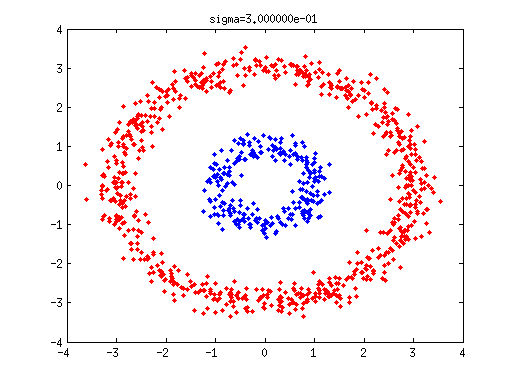
So consider turn the problem into graph clustering problem: connect the near point pairs in a “similarity graph” and run clustering. There’re several heuristic methods constructing the graph:
- $w_{i,j}=[\|x_i-x_j\|\le\epsilon]$
- $w_{i,j}=[x_j\in\mathrm{kNN}(x_i)\lor x_i\in\mathrm{kNN}(x_j)]$
- $w_{i,j}=\exp(-\|x_i-x_j\|^2/2)$
The formation of the graph, or say, adjacency matrix, is not unique, also there is no single canonical definition of graph clustering. But some specific version of this is equivalent to $k$-means. For now, let’s just forget about $k$-means and learn about different definitions of graph clustering and spectral clustering.
The general idea of graph clustering is to make intra-group edges having large weights and inter-group edges have small weights.
Definition 7. The Laplacian matrix for an undirected simple weighted graph $G$ is defined as: $$ (L_G)_{i,j}=\begin{cases}-w_{i,j},&i\ne j\\ d_i=\sum_jw_{i,j},&i=j\end{cases} $$ Theorem 2. Let $G$ be an undirected graph with non-negative weights, where $w_{i,j}=0$ means $(i,j)\notin E$. Multiplicity of $\lambda=0$ is the number of connected components, and $E_0=\span\set{1_{C_1},\cdots,1_{C_k}}$ where $C_i$s are the components and $1_S$ is the indicator vector.
Proof strategy. $$ v^\top Lv=\frac12\sum_{i,j}w_{i,j}(v_i-v_j)^2 $$ This looks useless—why not use DFS/BFS? The importance of Laplacian is that, it provides a continuous description of “connectivity”. For example, two cliques $K_n$ connected by few edges can be identified by a small but nonzero eigenvalue of the Laplacian. The eigenvalues of such Laplacian is $\set{0,n(\times 2n-3),(n+2\pm\sqrt{n^2+4n-4})/2}$, and $(n+2-\sqrt{n^2+4n-4})/2\approx 2/n$.
Definition 8. Spectral clustering is a heuristic method motivated by the spectral method under the ideal situation. It finds the eigenvectors corresponding to the bottom $k$ eigenvalues, denoted by $v_1,\cdots,v_k$, and run $k$-means on the $n$ rows of $\mat{v_1&\cdots&v_k}$, obtaining the clustering. Specifically, the bottom $k$ eigenvalues and eigenvectors are computed by power method on $L-\lambda_{\max}I$.
- Why is such algorithm reasonable, when the input is noisy graph from real-world data? There’re two perspectives:
- The “take bottom $k$ eigenvalues” step can be understood under another setting, which is the part focused on in class.
- There’re mathematical guarantees for the correct clustering of graphs deviating a small portion from the ideal disconnected graph.
Definition 9. The minimum ($k$-)cut problem (on a graph) is to find a partition of vertices $S_1,\cdots,S_k$, $$ \min.\sum_i\cut(S_i,\overline{S_i}) $$ This is not a good optimization objective because isolating single vertices is usually optimal.
Definition 10. The ratio cut problem is similar to the above one, but different at the goal $$ \min.\sum_i\frac{\cut(S_i,\overline{S_i})}{|S_i|} $$ Both mincut and ratiocut are NP-hard if $k$ is not constant.
Theorem 3. For $k=2$, minimizing ratio cut is equivalent to minimizing $v^\top Lv$, under some extra constraints on $v$.
Proof. Suppose the partition is $(S,\overline{S})$. Let $$ v_i^S=\begin{cases}\sqrt{\frac{|\overline S|}{|S|}},&i\in S\\ -\sqrt{\frac{|S|}{|\overline S|}},&i\notin S\end{cases} $$ then $$ (v_i^S)^\top L v_i^S=\frac12\sum_{i,j}w_{i,j}(v_i-v_j)^2=\sum_{i\in S,j\notin S}w_{i,j}\left(\sqrt{\frac{|\overline S|}{|S|}}+\sqrt{\frac{|S|}{|\overline S|}}\right)^2=\cut(S,\overline S)\left(\frac{|\overline S|}{|S|}+\frac{|S|}{|\overline S|}+2\right)=n\rcut(S,\overline{S}) $$ So the constraint is $v$ must be induced by some $S$.
Consider relaxing the constraint, finally we can get the goal $$ \min. v^\top Sv\quad\text{s.t. }v\perp 1,\|v\|_2=\sqrt n $$ This is the same goal as in definition 8.
Theorem 4. For general $k$, minimizing ratio cut is equivalent to minimizing $\tr(H^\top LH)$ where $H\in\R^{n\times k}$, s.t. $H^\top H=I$ and some other constraints.
Proof. Suppose the partition is $(S_1,\cdots,S_k)$. Let $$ H_{i,j}=\frac{1}{\sqrt{|S_j|}}[i\in S_j] $$ then $$ (H^\top LH)_{i,i}=\sum_{j\in S_i,k\notin S_i}\frac{w_{j,k}}{|S_i|}=\frac{\cut(S_i,\overline{S_i})}{|S_i|} $$ So $\tr(H^\top LH)=\rcut(S_1,\cdots,S_k)$ (of course only when $H$ is induced by some $(S_1,\cdots,S_k)$).
Theorem 5. The solution of $\min.\tr(H^\top LH)\text{ s.t. }H^\top H=I$ can be the matrix composed by the bottom $k$ eigenvectors of $L$.
Proof. The following proof has already appeared in the 计智应数 class.
Since $L$ is positive semidefinite, we can assume $L=W^\top W$. Let $W=\mat{w_1\\ \vdots\\w_n}$ and $H=\mat{h_1&\cdots&h_k}$, then $$ \tr(H^\top LH)=\tr((WH)^\top(WH))=\|WH\|_{\rm F}=\sum_i\left\lVert\proj_{\col(H)}w_i\right\rVert_2^2=\sum_i\sum_j\ip{w_i,h_j}^2 $$ This implies that, only $\col(H)$ really matters.
Now let’s use induction.
Let $V_k$ be the space spanned by the bottom $k$ eigenvector $\set{v_1,\cdots,v_k}$, and $V^\prime\ne V_k$ be another space of dimension $k$. By dimensionality, there exists unit vector $ v^\prime\in V^\prime\cap V_{k-1}^\perp$. It can be extended to an orthonormal basis of $V^\prime$, denoted as $\set{v_1^\prime,\cdots,v_{k-1}^\prime,v^\prime}$. Since the alternative definition of eigenvector is $$ v_k=\argmin_{v\perp v_1,\cdots,v_{k-1},\|v\|_2=1}v^\top L v $$ we have $v_k^\top Lv_k\le{v^\prime}^\top Lv^\prime$. Plus, by induction hypothesis, $$ \tr\left(\mat{v_1&\cdots&v_{k-1}}^\top L\mat{v_1&\cdots&v_{k-1}}\right)\le\tr\left(\mat{v_1^\prime&\cdots&v_{k-1}^\prime}^\top L\mat{v_1^\prime&\cdots&v_{k-1}^\prime}\right) $$ combining these two inequalities, we finally get $$ \tr\left(\mat{v_1&\cdots&v_{k-1}&v_k}^\top L\mat{v_1&\cdots&v_{k-1}&v_k}\right)\le\tr\left(\mat{v_1^\prime&\cdots&v_{k-1}^\prime&v^\prime}^\top L\mat{v_1^\prime&\cdots&v_{k-1}^\prime&v^\prime}\right) $$ Theorem 6. Denote the Laplacian of the ideal graph (clusters are completely disconnected) as $L_0$, and the actual noisy graph as $L=L_0+E$. Suppose by calculating the spectral decomposition and taking the bottom $k$ eigenvectors, we get $H$. Let $H^{*}$ be the real indicator of the clusters (induced by the partition), then there exists a rotation matrix $R$ and some constant $C$, $$ \|H-H^{*}R\|_{\rm F}\le C\frac{\|E\|}{\gamma} $$ where $\gamma$ is the eigengap and $C$ depends on the norm taken on $E$. Thus, running $k$-means on $H$ is valid, since right multiplying $R$ does not change the row pattern.
Obviously the proof will be some variant of the Davis–Kahan theorem.
Now let’s go back to $k$-means.
Theorem 7. $k$-means is equivalent to ratiocut.
Proof. Recall the optimization objective of $k$-means: $$ \sum_{i=1}^k\sum_{x\in S_i}\|x-\mu_i\|_2^2=\sum_x\|x\|_2^2-\sum_{i=1}^k|S_i|\|\mu_i\|_2^2\tag{1} $$ Let $X=\mat{x_1&\cdots&x_n}$, $H=\mat{1_{S_1}&\cdots&1_{S_k}}$, $D=\diag(|S_1|,\cdots,|S_k|)$. It can be easily verified that $XHD^{-1}=\mat{\mu_1&\cdots&\mu_k}$. So $(1)$ can be rewritten as $$ \tr\left(X^\top X-H^\top X^\top XHD^{-1}\right) $$ Here, $\tr(X^\top X)$ is constant and $\tr(H^\top X^\top XHD^{-1})=\tr(D^{-\alpha}H^\top X^\top XHD^{\alpha-1})$ for any $\alpha$ since we only consider trace. Here taking $\alpha=1/2$ can simplify the following derivation. So now the goal is $$ \max.\tr\left(D^{-1/2}H^\top X^\top XHD^{-1/2}\right)\quad\text{s.t. }H=\mat{1_{S_1}&\cdots&1_{S_k}},D=\diag(|S_1|,\cdots,|S_k|) $$ which is equivalent to $$ \max.\tr\left({\hat H}^\top X^\top X\hat H\right)\quad\text{s.t. }\hat H_{i,j}=\frac{1}{\sqrt{|S_j|}}[x_i\in S_j] $$
which is equivalent to $$ \min.\tr\left({\hat H}^\top L\hat H\right)\quad\text{s.t. }\hat H_{i,j}=\frac{1}{\sqrt{|S_j|}}[x_i\in S_j] $$ where $$ L_{i,j}=\begin{cases}-\ip{x_i,x_j},&i\ne j\\ \sum_{k\ne i}\ip{x_i,x_k},&i=j\end{cases} $$ is a valid Laplacian.
- In conclusion, the logic is
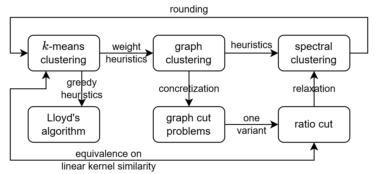
Stochastic Neighbor Embedding
Definition 11. Dimension reduction is the transformation of data from a high-dimensional space into a low-dimensional space so that the low-dimensional representation retains some meaningful properties of the original data. Here we focus on preserving neighborhoods. For example, PCA is a linear method for dimension reduction.
Definition 12. SNE is a nonlinear method for dimension reduction, motivated by NCA. NCA is supervised with labels, while SNE is unsupervised. SNE inherits the probability construction measuring nearness. For the given points $x_1\sim x_n$: $$ p_{j\mid i}=\frac{\exp\left(-\|x_j-x_i\|_2^2/2\sigma_i^2\right)}{\sum_{k\ne i}\exp\left(-\|x_k-x_i\|_2^2/2\sigma_i^2\right)},p_{i\mid i}=0 $$ Let $y_i=f(x_i)$ be the reduced points (usually 2D/3D), $$ q_{j\mid i}=\frac{\exp\left(-\|y_j-y_i\|_2^2\right)}{\sum_{k\ne i}\exp\left(-\|y_k-y_i\|_2^2\right)},p_{i\mid i}=0 $$ The loss is defined as $$ L=\sum_i\mathrm{KL}(p_i\parallel q_i)=\sum_i\sum_jp_{j\mid i}\log\frac{p_{j\mid i}}{q_{j\mid i}} $$ The parameters $\sigma_i$ controls perplexity: $$ \mathrm{perp}(p_i)=2^{H(p_i)},H(p_i)=-\sum_jp_{j\mid i}\log p_{j\mid i} $$
- Higher perplexity → more uniform $p_i$ → larger $\sigma_i$. Higher perplexity → more effective neighbors considered → denser view.
- The reason using separate $\sigma_i$s is because different $x_i$s may be in dense/sparse regions, and we want to fix the number of neighbors considered across all the points.
- In low dimension, $\sigma$ is not used because: 1. We shouldn’t use different $\sigma_i$ for each point since we want the dense clusters to look dense and the sparse clusters to look sparse. 2. A uniform $\sigma$ is useless because we can just scale the points.
Definition 13. t-SNE is an adjusted version of SNE, solving crowding problem. It applies the following modification: $$ p_{ij}=\frac{p_{j\mid i}+p_{i\mid j}}2 $$
$$ q_{ij}=\frac{\left(1+\|y_i-y_j\|_2^2\right)^{-1}}{\sum_k\sum_{l\ne k}\left(1+\|y_k-y_l\|_2^2\right)^{-1}},q_{ii}=0 $$
$$ L=\sum_{i\ne j}p_{ij}\log\frac{p_{ij}}{q_{ij}} $$
Here $q$ is calculated using Student’s $t$ distribution with one degree of freedom (which is also the Cauchy distribution). Its benefit is that it’s heavy-tailed. Relative differences in distance are diluted.
- Here I use an example to illustrate the advantage of using a heavy-tailed distribution. Since in high dimensions there’s a scaling factor $\sigma_i$, considering relative density may be more convincing. For some point $x$, there’re $2^d$ times more points within distance $2r$ from $x$ than within distance $r$. In low dimensions, this would require the same ratio between the $2\sigma_ir$ neighborhood and the $\sigma_ir$ neighborhood, which is impossible since the space ratio is only $2^2$ or $2^3$. But under Student’s $t$ distribution, the ratio between the two corresponding distances in low dimensions is far larger than $2^2$ or $2^3$.
Visualization of t-SNE is available here.
Self-Supervised Learning
The three greatest ideas of ML are:
- Converting discrete quantities into continuous.
- Sampling a small batch of data within the whole data space, which can be regarded as some kind of general SGD.
- Caring about relations, rather than absolute “meanings”. As a saying goes, a French pupil may not know $2+3=5$, but he must know $2+3=3+2$. In self-supervised learning, the model is not explicitly told the labels of images, but it learns to recognize semantic meanings by being trained to predict the relationship between two images.
Contrastive Learning
This part centers around the paper Contrastive Learning Is Spectral Clustering On Similarity Graph.
Definition 1. Contrastive learning is a self-supervised learning method that makes a model learn to understand data by training on similar and dissimilar data pairs. Specifically, the approach trains a neural network to map a set of objects into an embedding space, ensuring that similar objects are closely positioned while dissimilar objects remain far apart.
Definition 2. SimCLR is a simple framework for contrastive learning of visual representations. It trains a neural network $f:\sp X\to\sp Z$ that maps an image from pixel space to feature space. The loss is defined as follows: For each original image $x_i$, augment it to two images $\tilde x_{2i-1}$ and $\tilde x_{2i}$. The augmentation method is sampled from an augmentation function class $\sp T$. Let $z_i=f(\tilde x_i)$. The loss is InfoNCE loss $$ L=\sum_i-\log\frac{\exp\left(-\|z_i-z_{j=i-(-1)^i}\|^2/2\tau\right)}{\sum_{k\ne i}\exp\left(-\|z_i-z_k\|^2/2\tau\right)} $$ Definition 3. To analyze SimCLR, here we define a theoretical model, which is some kind of generalization. These are the objects in the model:
- $\pi$, the similarity matrix in the original space, having dimension $|\sp X|\times|\sp X|$. $\pi$ is defined by the augmenting strategy, and is not explicitly written out since $|\sp X|$ is usually large (like $256^{3wh}$). In SimCLR, $\pi_{i,j}$ is the probability that image $i$ and $j$ being sampled together. $\pi$ can sometimes be regarded as a stochastic matrix. $\pi$ is not necessarily symmetric, although in SimCLR it is.
- $K_Z$, the similarity matrix in the feature space. The definition is ${K_Z}_{i,j}=\ip{\phi(f(X_i)),\phi(f(X_j))}_{\sp H}$, where $\phi:\sp Z\to\sp H$ is the “feature map” (this “feature” is unrelated to the semantic feature of the images) and $\sp H$ is the reproducing kernel Hilbert space. The motivation here is, we are not limited to using $\ell_2$-norm in the feature space, but we can define more complex similarity function as long as it satisfies some basic properties.
- The sampling process. Each matrix defines a weighted graph, and the idea here is to sample a subgraph $W$. The subgraph must satisfy some property, expressed by an indicator function $\Omega:\sp W\to \set{0,1}$. Here, we consider the graph to be directed, and specify $\Omega(W)$ to be “every vertex in $W$ has out degree $1$”. Note that it’s not SimCLR anymore. Now the distribution is defined as $\Pr[W;\pi]\propto\Omega(W)\prod_{(i,j)}\pi_{i,j}^{W_{i,j}}$ (define $0^0=1$). Under the assumption that each row of $\pi$ sums to $1$ and the specification of $\Omega$, $\propto$ can be replaced by $=$. Note that this “probability” is not even similar to normal subgraph sampling since in normal sampling, $W_{i,j}=0$ should contribute $1-\pi_{i,j}$ to the probability.
- The loss. We use cross entropy function to compare $\pi$ and $K_Z$: $H_{\pi}^k(Z)=-\Ex_{W_X\sim\Pr[\cdot;\pi]}(\log\Pr[W_Z=W_X;K_Z])$. Here $W_X$ is sampled according to $\pi$ and $W_Z$ is sampled according to $K_Z$. $k$ on the superscript is the kernel function $\ip{\phi(\cdot),\phi(\cdot)}_{\sp H}$.
- The high-level mechanism of contrastive learning is that $\pi$ gives guidance, a sketch of representation learning, which is not complete (for example, if images $i$ and $j$ represent two different dogs of the same breed, $\pi_{i,j}=0$ since they cannot be obtained by augmentation), and $f$ learns the feature and automatically generalizes to other real-world images by some generalization guarantee. Contrastive learning is powerful because it does not require labels or a huge amount of data, but depends solely on data synthesis. However, I think it’s unimpressive that the following theory does not provide a more accurate description of this intuition.
Theorem 1. Minimizing $H_\pi^k(Z)$ is equivalent to (a modified/idealized version) SimCLR, and is also equivalent to spectral clustering on $\pi$.
Proof. Equivalence to SimCLR: $$ \eq{ H_\pi^k(Z)&=-\Ex_{W_X\sim\Pr[\cdot;\pi]}\left(\log\prod_i\Pr[{W_Z}_i={W_X}_i;K_Z]\right)\\ &=-\Ex_{W_X\sim\Pr[\cdot;\pi]}\left(\sum_i\log\Pr[{W_Z}_i={W_X}_i;K_Z]\right)\\ &=-\sum_i\Ex_{j\sim\pi_{i,\cdot}}\left(\log\frac{{K_Z}_{i,j}}{\sum_k{K_Z}_{i,k}}\right)\\ &=-\sum_i\Ex_{j\sim\pi_{i,\cdot}}\left(\log\frac{k(f(X_i),f(X_j))}{\sum_tk(f(X_i),f(X_j))}\right) } $$ Comparing with the SimCLR’s objective, the only difference is that here, for every possible image in $\sp X$, we sample its counterpart, while in SimCLR a subgraph is considered.
Equivalence to spectral clustering:
Denote $R(Z)=\sum_{W}\Omega(W)\prod_{(i,j)}{K_Z}_{i,j}^{W_{i,j}}$. $$ \eq{ \log\Pr[W_Z=W_X;K_Z]&=\log\frac{\prod_{(i,j)}{K_Z}_{i,j}^{{W_X}_{i,j}}}{R(Z)}\\ &=\sum_{i,j}{W_X}_{i,j}\log K(Z_i,Z_j)-\log R(Z)\\ &=-\sum_{i,j}{W_X}_{i,j}\frac{\|Z_i-Z_j\|^2}{2\tau}-\log R(Z)\\ &=-\frac{1}{\tau}\tr(Z^\top L(W_X)Z)-\log R(Z)\\ \implies-\Ex_{W_X\sim\Pr[\cdot;\pi]}(\log\Pr[W_Z=W_X;K_Z])&=-\frac1\tau\tr(Z^\top L(\pi)Z)+\log R(Z) } $$ This is the optimization objective of ratiocut, with that $Z^\top Z=1$ constraint replaced by a regularization term $\log R(Z)$.
- SimCLR only sample a subgraph with $2n$ vertices and $n$ edges. The paper Momentum Contrast for Unsupervised Visual Representation Learning attempted to train on larger subgraphs (more negative samples) and found that the model performs better with larger subgraph. This is nontrivial since this contrasts to normal minibatch sampling, where increasing minibatch size does not significantly improve the performance.
Misc
Rotary Position Embedding
Don’t ask me why it is taught in this course. I don’t know.
In order to encode position information and add it to the word embeddings in transformer, consider RoPE: $$ q_m^\prime=q_mR_m=x_mW_qR_m,k_n^\prime=k_nR_n=x_nW_kR_n,q_m^\prime{k_n^\prime}^\top=x_mW_qR_{m-n}W_k^\top x_n^\top=q_mR_{m-n}k_n^\top $$ (Here $x_m$ is row vector) where $$ R_m=\mat{\cos m\theta_0&-\sin m\theta_0&\cdots&0&0\\ \sin m\theta_0&\cos m\theta_0&\cdots&0&0\\ \vdots&\vdots&\ddots&\vdots&\vdots\\ 0&0&\cdots&\cos m\theta_{\frac d2-1}&-\sin m\theta_{\frac d2-1}\\ 0&0&\cdots&\sin m\theta_{\frac d2-1}&\cos m\theta_{\frac d2-1}},\;\theta_i=10000^{-\frac{2i}d} $$ It can be understood as adding signals at different scales of frequency (so that the model can distinguish different orders of distances). This matrix is not arbitrarily designed, it has several advantages:
- Light computation cost.
- Preserving length.
- No need to use complex numbers (compared to $\diag(\e^{\i m\theta_0},\cdots,\e^{i m\theta_{\frac d2-1}})$).
Note that we don’t want $m\theta_{\frac d2-1}\ge 2\pi$, otherwise it will cause “aliasing”—$R_m$ fails to help the model identify the distance uniquely (although $R_0\ne R_{20000\pi}$, their lowest frequency signal will be the same / very close geometrically, confusing the model).
Robust Machine Learning
Definition 1. An adversarial example is an instance with small, intentional feature perturbations that cause a machine learning model to make a false prediction (taken from this book). Below is an example from the paper Explaining and Harnessing Adversarial Examples illustrating this kind of example:
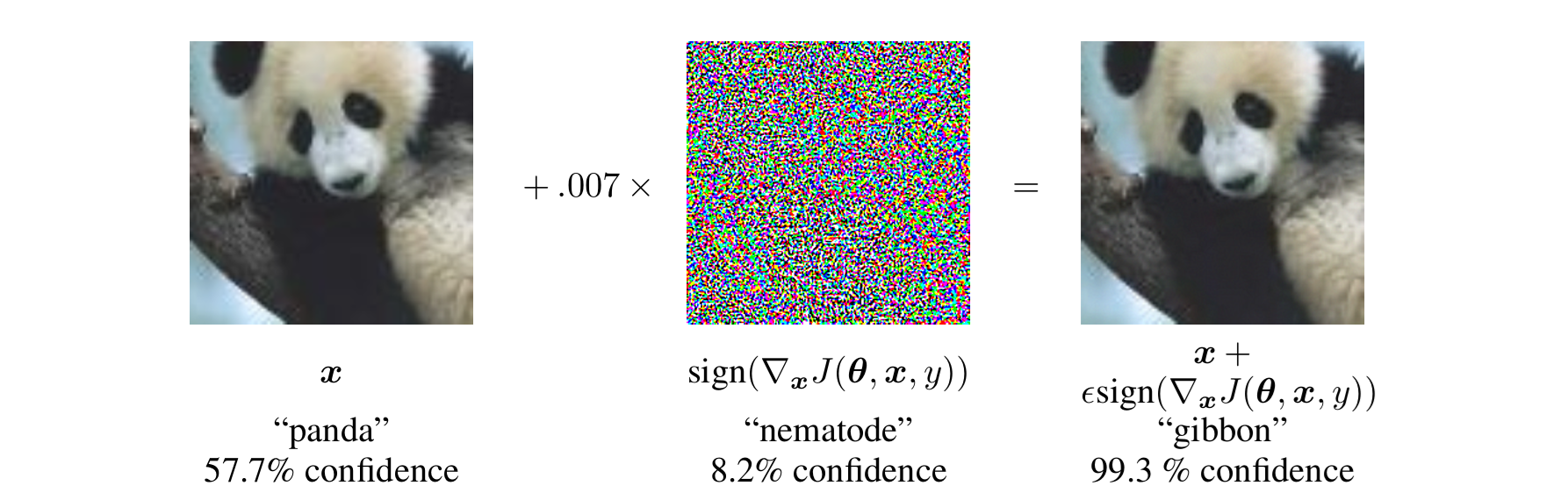
Definition 2. Adversarial attacks can be defined as an optimization problem. Recall the original supervised learning goal: $$ \min_\theta.\ell(f_\theta(x),y) $$ Here the goal is changed to $$ \max_\delta.\ell(f_\theta(x+\delta),y)\quad\text{s.t. }\delta\in\Delta $$ where $\Delta$ is a small region near $0$. Of course it can be optimized by GD methods, with constraints, called PGD: $$ \delta_{t+1}=\proj_{\Delta}\left(\delta_t+\eta\nabla_x\ell(f_\theta(x+\delta_t,y))\right) $$ but the problem is that, since such optimization is “unexpected”, the loss landscape w.r.t. $\delta$ may be pathological. Some components of the gradient may be extremely small, but drastically change after some steps. So, we may want to simply set $\eta\to\infty$ and $\Delta=\set{\delta\mid\lVert\delta\rVert_\infty\le\epsilon}$ (If use $\ell_2$ norm, a small fraction of components will dominate). Under this settings, $\delta$ will simply be $\epsilon\sgn\left(\nabla_x\ell(f_\theta(x),y)\right)$. This is called fast gradient sign method, or FGSM. Using this as a subroutine, we can run multiple steps of FGSM, each step using a small $\epsilon$ and set a overall larger $\epsilon$. This has no mathematical guarantee but empirically producing useful adversarial examples.
The paper Universal and Transferable Adversarial Attacks on Aligned Language Models showcases some hilarious adversarial examples jailbreaking LLMs.
Definition 3. Adversarial training is training the model to be robust against adversarial examples. The goal is: $$ \min_\theta.\Ex_{x,y}\left(\max_{\delta\in\Delta}\ell(f_\theta(x+\delta),y)\right) $$ which is seemingly hard to optimize.
Theorem 1 (Danskin). Let $g(y)=\max_{x\in Q}f(x,y)$ where $Q$ is compact, $f$ is continuous and $\frac{\p}{\p y}f(x,y)$ is continuous, $$ g^\prime(y)=\max_{x^{*}\in\argmax_{x\in Q}f(x,y)}\frac{\p}{\p y}f(x_{*},y) $$ If $y$ is multivariate, for any direction $v$, $$ \nabla_vg(y)=\max_{x^{*}\in\argmax_{x\in Q}f(x,y)}\nabla_vf(x_{*},y) $$ Now we do two steps of relaxation: first we only consider one of the $\argmax$, second we do not require $x^{*}$ to be exact. Then we just need to solve this: $$ \frac1N\frac{\p}{\p\theta}\ell(f_\theta(x_i+\delta_i^{*}),y_i)=0 $$ where $\delta_i^{*}$ is an adversarial example constructed for $(x_i,y_i)$, approximating $\argmax$. In this way, we can do GD just like normal classification training, only adding an adversarial construction step before every minibatch update. The key point here is recomputing $\delta_i^{*}$ every step. By experiment, if one uses the same $\delta_i^{*}$ across all update steps, the outcome won’t be good.
Other than directly training robust methods, there’re several shortcuts, or hotfixes, but they eventually turned out to be vulnerable.
Definition 4. FGSM and PGD rely on gradients. Obfuscated gradients are defense methods that try to protect a neural network by breaking or hiding the gradient information that attackers use:
- Shattered gradients, like including input discretization, JPEG compression, thresholding, etc. The main idea is to introduce a nondifferentiable “preprocessing” function $g(x)\approx x$, and feed $g(x)$ into the non-robust model $f(x)$.
- Stochastic gradients, to introduce randomness during inference, like $g(x)=x+(\delta\sim\Nd)$, or random dropout.
- Exploding and vanishing gradients, to make the neural network extremely deep.
But these methods are just giving so-called “false sense of security”. Advanced attackers can bypass them by:
- Approximating $\nabla_x(f_\theta\circ g)(x)$ by $(\nabla_xf_\theta)\circ g(x)$.
- Taking average of the gradients over many random trials.
Leaving only the actually robustly-trained model alive. Even cooler, authors of the paper Synthesizing Robust Adversarial Examples built real-world objects whose photos from different perspectives all successfully confused non-robust models.
Definition 5. A simple provable robust certificate was introduced in class. A robust model $g(x)$ is obtained by augmenting the original model $f(x)$ by $$ p(x)_{\hat y}=\int_\delta[f(x+\delta)=\hat y]w(\delta)\d\delta $$ and $g(x)=\text{majority or absolute majority of }p$. Here $w(\delta)$ is a probability weight function like $[\|\delta\|_2\le r]/V_r$ or Gaussian, and the integral is evaluated using sampling in practice. Under this setting, let $y$ be the correct label, if $p(x)_y$ is large, it is mathematically guaranteed that in some neighborhood of $x$, the prediction $g(x^\prime)$ is always correct.
Theorem 2. For a data $(x,y)$, denote $c(x^{\prime})=p(x^{\prime})_y$. Knowing $c(x)$, the lower bound of $c(x+\delta)$ can be calculated as follows: Sort all the points $y$ by $k(y)=\frac{w(y-x)}{w(y-x-\delta)}$. Find a threshold $T$ that $\int_{k(y)\ge T}w(y-x)\d y=c(x)$, then $$ c(x+\delta)\ge\int_{k(y)\ge T}w(y-x-\delta)\d y $$ This is called greedy filling and the correctness is self-evident.
If $w(\delta)=[\|\delta\|_2\le r]/V_r$, then by first filling $B_r(x)\setminus B_r(x+\delta)$ then $B_r(x)\cap B_r(x+\delta)$, we can see $c(x+\delta)=\max\set{c(x)-\lvert B_r(x)\setminus B_r(x+\delta)\rvert/V_r,0}$.
If $w(\delta)$ is Gaussian, the contours of $k(y)$ are hyperplanes and $c(x+\delta)=\Phi(\Phi^{-1}(c(x))-\|\delta\|_2)$ where $\Phi$ is the CDF.
Hyperparameter
Hyperparameter tuning is usually hard because the function doesn’t have nice structure and the queries have high (real-world) costs. Several techniques are introduced in class, including:
| Approach | Theorem |
|---|---|
| Graduate student Descent | / |
| Bayesian inference | 1 |
| Gradient Descent | 2, 3 |
| random search / grid search | / |
| multi-armed bandit based algorithms | 4, 5 |
| neural architecture search | / |
When we have no prior knowledge of the loss landscape in hyperparameter space, the best choice is random search.
Definition 1. Gaussian process is a type of infinite-dimensional Gaussian distribution. A Gaussian process, denoted as $f$, is defined on a continuous domain $D$. For every $x\in D$, $f(x)$ follows Gaussian distribution. Furthermore:
- $\forall x_1,\cdots,x_n\in D$, their joint distribution is also a Gaussian.
- There’s a covariance function $K(\cdot,\cdot)$ defining the process. We know that a multivariate Gaussian can be defined by its covariance matrix. In the infinite-dimensional case, $\forall x_1,x_2\in D$, $\Cov(x_1,x_2)=K(x_1,x_2)$. Obviously we usually consider nearer points to have higher covariance.
- Here we also require $\Ex(f(x))=0$ for every $x$.
Definition 2. For general hyperparameter optimization, one approach is to use Bayesian inference. We use a Gaussian process over the hyperparameter space to model the prior. After a sample is given, update the posterior, and use the posterior distribution to guide the selection of the next sample point.
Theorem 1. The posterior of Gaussian process has analytical form. Given $m$ observations $(x_i,y_i)$, $$ f(x)\sim\Nd\left(k_{*}^\top\Sigma^{-1}y,K(x,x)-k_{*}^\top\Sigma^{-1}k_{*}\right)\text{ where }k_{*}=\mat{K(x_1,x)\\ \vdots\\K(x_m,x)},y=\mat{y_1\\ \vdots\\y_m} $$ GP methods become ineffective when the dimension is large (more than tens), due to sample inefficiency and kernel learning failures in high-dimensional spaces.
For some continuous hyperparameters, we can use GD, that is, computing the gradient of the loss w.r.t. the hyperparameters. Take GD process as an example. To optimize $\eta$, first recall the gradient update: $$ w_{t+1}=w_t-\eta\nabla^\top L(w_t) $$ The naïve way to calculate $\nabla_\eta L$ is storing every $w_t$, which takes $\O(Tdw)$ ($w$ is the size of a word) space.
Theorem 2. For gradient descent, we can maintain $\nabla_\eta L$ alongside the gradient update.
Proof. Here I don’t follow the shape convention, so I explicitly use $\nabla^\top$ to denote column vector-shaped gradient. First, $$ \nabla_\eta L(w_T)=\nabla L(w_T)\cdot\nabla_\eta w_T $$ where $\nabla L(w_T)=(\nabla L)(w_T)$. Then, $$ \eq{ \nabla_\eta w_T&=\nabla_\eta(w_{T-1}-\eta\nabla^\top L(w_{T-1}))\\ &=\nabla_\eta w_{T-1}-\nabla^\top L(w_{T-1})-\eta\nabla_\eta\nabla^\top L(w_{T-1})\\ &=\nabla_\eta w_{T-1}-\nabla^\top L(w_{T-1})-\eta\nabla^2L(w_{T-1})\nabla_\eta w_{T-1}\\ &=(I-\eta\nabla^2L(w_{T-1}))\nabla_\eta w_{T-1}-\nabla^\top L(w_{T-1}) } $$
which is a first-order recurrence. This is called Forward-Mode Differentiation. The problem with it is that, if there’re not just one, but thousands of hyperparameters $\eta_1,\cdots,\eta_k$, we need to store $\nabla_{\eta_i}w_T$ for each $\eta_i$, costing $\O(kdw)$ space.
Definition 3. The process of momentum gradient descent (with variable learning rate) is:
- First initialize $w_0$.
- Every step let $g_t=\nabla_{w_t}L(w_t,\theta,t)$, where $\theta$ contains the configuration of the training loss. Then $v_{t+1}=\gamma_tv_t-(1-\gamma_t)g_t$, $w_{t+1}=w_t+\alpha_tv_{t+1}$.
- Note that this formula is slightly different from the one presented in class: in the slides it is $w_{t+1}=w_t+\alpha_tv_t$. So the following recurrence formulas are also slightly different.
Theorem 3. Using momentum gradient descent, we can trace back to the gradient of intermediate parameters with respect to the hyperparameters, from the final state.
Proof. The hyperparameters are: $w_1$, $\theta$, $\gamma_t$, $\alpha_t$. Denote the test loss as $f(w_T)$. Now we can calculate the gradients by chain rule. Initially we only have $v_T$, $w_T$ and $\nabla_{w_T}f(w_T)$.
- $w_t=w_{t+1}-\alpha_tv_{t+1}$
- $g_t=\nabla_{w_t}L(w_t,\theta,t)$
- $v_t=(v_{t+1}+(1-\gamma_t)g_t)/\gamma_t$
- $\nabla_{\alpha_t}f(w_T)=\nabla_{w_{t+1}}f(w_T)\nabla_{\alpha_t}w_{t+1}=\nabla_{w_{t+1}}f(w_T)v_{t+1}$
- $\nabla_{\gamma_t}f(w_T)=\nabla_{v_{t+1}}f(w_T)\nabla_{\gamma_t}v_{t+1}=\nabla_{v_{t+1}}f(w_T)(v_t+g_t)$
- $\nabla_\theta f(w_T)\xleftarrow{+}\nabla_{v_{t+1}}f(w_T)\nabla_{g_t}v_{t+1}\nabla_\theta g_t=-\nabla_{v_{t+1}}f(w_T)(1-\gamma_t)\nabla_\theta\nabla_{w_t}L(w_t,\theta,t)$
- $\nabla_{w_t}f(w_T)=\nabla_{v_{t+1}}f(w_T)\nabla_{g_t}v_{t+1}\nabla_{w_t}g_t=-\nabla_{v_{t+1}}f(w_T)(1-\gamma_t)\nabla_{w_t}\nabla_{w_t}L(w_t,\theta,t)$
- $\nabla_{v_t}f(w_T)=\nabla_{w_t}f(w_T)\nabla_{v_t}w_t+\nabla_{v_{t+1}}f(w_T)\nabla_{v_t}v_{t+1}=\nabla_{w_t}f(w_T)\alpha_{t-1}+\nabla_{v_{t+1}}f(w_T)\gamma_t$
This procedure is called Reverse-Mode Differentiation, or simply backpropagation.
To analyze the space used by this method, we need to take precision into consideration. If we use floating point expression and keep dividing $v$ by $\gamma$, after a number of time, $v$ will be full of noise produced by the precision error which is initially tiny. If we use fractional expression, by information theory we need to store at least $\O(T\log\gamma^{-1})$ bits, which is far less than storing every $w_t$, or using forward-mode differentiation.
Definition 4. The best arm identification problem is to identify the one with the maximum expectation, among $n$ random variables $X_1,\cdots,X_n$, under limited number of sampling of these variables.
Definition 5. The successive halving (SH) algorithm is as follows: Let the budget be $B$. Run $\log_2n$ rounds with round $i$ sampling each remaining variables $\frac{2^iB}{n\log_2n}$ times and preserving the half with the largest empirical averages. Empirical average is defined as the average of sampling results across all the previous rounds. For hyperparameter tuning, SH is simplified to just looking at the current loss.
Theorem 4. Assume $\Ex(X_1)>\Ex(X_2)\ge\cdots\ge\Ex(X_n)$. Let $H_2=\max_{i>1}i/(\Ex(X_1)-\Ex(X_i))^2$. $$ \Pr\left[\text{SH returns the best arm with }B=\O\left(H_2\log n\log\frac{\log n}\delta\right)\right]\ge 1-\delta $$ Theorem 5. For hyperparameter tuning, assume $v_i=\lim_{t\to\infty}\ell_i(t)$. Let $\gamma_i(t)=\max_{t^\prime\ge t}|\ell_i(t^\prime)-v_i|$ and $\gamma^{-1}(\alpha)=\min\set{t\mid \gamma(t)\le\alpha}$. Assume $v_1<v_2\le\cdots\le v_n$ and let $\bar\gamma(t)=\max_i\gamma_i(t)$. SH returns the best arm if $$ B\ge 2\log_2n\left(n+\sum_{i>1}\bar\gamma^{-1}\left(\frac{v_i-v_1}{2}\right)\right) $$
Interpretability
Interpretability is the ability to explain why a machine learning model makes a specific decision rather than just accepting its output as a black box. Good interpretability typically involves attribution methods, which assign weights to input variables to show how much each factor influenced the final result.
Definition 1. LIME, Local Interpretable Model-agnostic Explanations, is a technique that approximates any black box machine learning model with a local, interpretable model to explain each individual prediction (taken from this post). The intuition is, although the whole prediction landscape is nonlinear, a linear interpretation around some certain point that we care about is plausible and viable. Here are the notations:
- $f$ is the trained model and $g$ is a linear model, both mapping the inputs to some labels. When we focus on some specific label, $f$ may stand for the corresponding component of the predicted distribution.
- $\Pi_x$ is a sampling mechanism near $x$. It assigns greater values to those samples near $x$.
- $L(f,g,\Pi_x)$ is the loss of linear model $g$ on the sampled points based on $\Pi_x$, with reference to $f$.
- $\Omega(g)$ measures the complexity of $g$, which acts as a regularization term in the objective function.
The final objective is $$ \min_g. L(f,g,\Pi_x)+\Omega(g) $$ For example:
- $\Omega(g)=[\|w\|_0>s]\cdot+\infty$, which should be converted to LASSO-like soft regularizer.
- $\Pi_x(z)=\exp(-D(x,z)^2/\sigma^2)$ where $D$ is some distance metric.
- $L(f,g,\Pi_x)=\sum_z\Pi_x(z)\cdot(f(z)-g(z))^2$.
Definition 2. LIME explains an image classification by the following process:
- Use a segmentation algorithm to partition the image into $m$ superpixels $S_1,\cdots,S_m$.
- Sample images by sampling binary vectors $z\in\set{0,1}^m$. The corresponding image is obtained by masking those superpixels $S_i$ for $z_i=0$, denoted as $\sum z_iS_i$ in shorthand.
- Train, say $g_\theta(z)=\sigma(\theta^\top z+b)$, by $L(f,g_\theta,\Pi_x)=\sum_z\exp(-(\text{\# of 0s in }z)^2/\sigma^2)\cdot(f(\sum z_iS_i)-g_\theta(z))$.
- Recognize the top-$k$ components of $\theta$ as the indicators responsible for the label.
- Why don’t simply use ablation? Because LIME takes interactions between components, and nonlinearity into account. Consider an extreme example: A dog is classified only by its two ears $S_1,S_2$, but either of its ears is enough. So $f(S_1+S_2)=1$ but also $f(S_1)=f(S_2)=1$. Ablation fails to account for this, but in LIME we face such equation set, so that the importance of both ears is equally stressed: $$ \begin{cases} \sigma(\theta_1+\theta_2+\text{others})\approx 1\\ \sigma(\theta_1+\text{others})\approx 1\\ \sigma(\theta_2+\text{others})\approx 1\\ \sigma(\text{others})\approx 0 \end{cases} $$
- In practice we don’t always sample by replacing part of the input by zero/black, but rather do some small perturbation. This will expose the deficiencies of LIME: it only finds a tangent hyperplane, and the gradient is local while the information itself is not (think of vanishing gradient problem). LIME also suffers from other drawbacks e.g. instability, lack of interaction handling etc.
The following part centers around the paper Axiomatic Attribution for Deep Networks.
Definition 3. The Integrated Gradients Algorithm attributes the contribution of each component $i$ of the input $x$ to the following integral: $$ \mathrm{IntegratedGrads}_i(x)=(x_i-x_i^\prime)\int_0^1\frac{\p f(x^\prime+\alpha(x-x^\prime))}{\p x_i}\d\alpha $$ where $x^\prime$ is the baseline, for example a pure black image in the case of image classification. In practice the integral is approximated by some finite element method.
Theorem 1 (informal). The Integrated Gradients Algorithm is the only algorithm that satisfies the following properties (or axioms, in the original paper):
- Sensitivity.
- If for every input and baseline that differ in one feature but have different predictions then the differing feature should be given a non-zero attribution.
- If the function implemented by the deep network does not depend (mathematically) on some variable, then the attribution to that variable is always zero.
- Implementation invariance. The attributions should always be identical for two functionally equivalent networks, i.e. the input-output mappings are the same while the implementation could possibly differ.
- Completeness. The attributions add up to the difference between the output of $f$ at the input $x$ and the baseline $x^\prime$.
- Linearity. The attributions for $af_1+bf_2$ should be the weighted sum of the attributions for $f_1$ and $f_2$ with weights $a$ and $b$ respectively.
- Symmetry-preserving. If two input variables are symmetric w.r.t. $f$ (e.g. $f(x,y)=\sigma(x+y)$), they should receive identical attributions.
Definition 4. The SHAP algorithm is a method that attributes contribution of every discrete element of the input, while following the similar properties of IG algorithm as listed above. For some prediction $f(\set{x_1,\cdots,x_n})$, SHAP assigns $$ \phi_i(f)=\sum_{S\subseteq[n]\setminus\set{i}}\frac{|S|!(n-|S|-1)!}{n!}(f(S\cup\set{i})-f(S)) $$ The combinatorial meaning is enumerating every permutation of $x_1,\cdots,x_n$, adding the elements following the permutation and averaging the change of prediction. For element $i$, there are $|S|!(n-|S|-1)!$ permutations of the form $S,i,[n]\setminus(S\cup\set{i})$, all contributing $f(S\cup\set{i})-f(S)$.
Both IG and SHAP focus on global attribution, so sometimes they exhibit poor local fidelity.
Selective Exercises
Problem 1. Prove that for $f\in\fF^1(\R^n)$ and $g\in\fF^0(\R^n)$, at $x_{*}=\argmin_x\set{f(x)+g(x)}$, $\forall x$, $g(x)\ge g(x_{*})-\ip{\nabla f(x_{*}),x-x_{*}}$. Avoid using subgradient.
Solution (wmy). Let $x=x_{*}+tu$ where $\|u\|=1$. By Taylor expansion, $$ f(x)=f(x_{*})+t\ip{\nabla f(x_{*}),u}+\omicron(t) $$ Also $$ f(x)+g(x)\ge f(x_{*})+g(x_{*}) $$ so $$ g(x)-g(x_{*})\ge -t\ip{\nabla f(x_{*}),u}+\omicron(t)\implies\frac{g(x_{*}+tu)-g(x_{*})}t\ge-\ip{\nabla f(x_{*}),u}+\omicron(1) $$ We know that $(g(x_{*}+tu)-g(x_{*}))/t$ is monotone, so $$ \frac{g(x_{*}+tu)-g(x_{*})}{t}\ge \lim_{t^\prime\to 0^{*}}\frac{g(x_{*}+t^\prime u)-g(x_{*})}{t^\prime}\ge -\ip{\nabla f(x_{*}),u} $$ Problem 2. In MD, if we add a constraint on $x$, that is, consider a convex set $Q$, $x_{t+1}=\argmin_{y\in Q}\set{\cdots}$. How to modify the proof, to get the same result?
Solution. Recall that $x_{t+1}=\argmin_{y}\set{\ip{\eta\nabla f(x_t),y-x_t}+V_{x_t}(y)}$. The error appears at line 2/3 in the proof of theorem 15: $$ \ip{\eta\nabla f(x_t),x_{t+1}-x_{*}}=\ip{-\nabla V_{x_t}(x_{t+1}),x_{t+1}-x_{*}} $$ For arbitrary $Q$, it’s hard to write the Lagrange multiplier. Here’s a way only using properties of convex set: Let $g(y)=\ip{\eta\nabla f(x_t),y-x_t}+V_{x_t}(y)$, $h(\alpha)=g(x_{t+1}+\alpha(x_{*}-x_{t+1}))$. Since $x_{t+1}$ is argmin, $h^\prime_+(0)\ge 0$: $$ \ip{\nabla g(x_{t+1}),x_{*}-x_{t+1}}=\ip{\eta\nabla f(x_t)+\nabla V_{x_t}(x_{t+1}),x_{*}-x_{t+1}}\ge 0 $$ i.e. $$ \ip{\eta\nabla f(x_t),x_{t+1}-x_{*}}\le\ip{-\nabla V_{x_t}(x_{t+1}),x_{t+1}-x_{*}} $$ Problem 3. On probability vectors, define $w(x)=\sum x^i\log x^i$, $V_x(y)=\sum y^i\log\frac{y^i}{x^i}$. Prove that $V_x(y)\ge\frac12\|x-y\|_1^2$, that is, it is $1$-strongly convex w.r.t. to $1$-norm.
Solution 1 (mjy). By Taylor expansion, $\exists\xi=x+\theta(y-x)$, $$ V_x(y)=w(y)-w(x)-\ip{\nabla w(x),y-x}=\frac12(y-x)^\top\nabla^2w(\xi)(y-x) $$ Surprisingly, $$ \nabla^2 w(\xi)=\diag\left(\frac{1}{\xi^1},\cdots,\frac{1}{\xi^d}\right) $$ by Cauchy inequality, $$ (y-x)^\top\nabla^2w(\xi)(y-x)=\sum_{i=1}^d\frac{(y^i-x^i)^2}{\xi^i}=\left(\sum_{i=1}^d\frac{(y^i-x^i)^2}{\xi^i}\right)\left(\sum_{i=1}^d\xi^i\right)\ge\left(\sum_{i=1}^d|y^i-x^i|\right)^2=\|x-y\|_1^2 $$
Solution 2 (standard proof of Pinsker’s inequality that can be generalized to infinite-dimension case). First, for $0 \le p, q \le 1$, let $f(p,q) = q\log\frac{q}{p} + (1-q)\log\frac{1-q}{1-p} - 2(q-p)^2$. $$ \frac{\partial f}{\partial p} = -\frac{q}{p} + \frac{1-q}{1-p} + 4(q-p) = (q-p)\left(4-\frac{1}{p(1-p)}\right)\begin{cases}\le 0,&q\le p\\ \ge 0,&q\ge p\end{cases} $$ when $p=q$, $f(p,q)=0$. So $f(p,q) \ge 0$. Now, $$ \eq{ \sum_{i=1}^n y_i \log\frac{y_i}{x_i} &= \sum_{y_i \le x_i} y_i \log\frac{y_i}{x_i} + \sum_{y_i > x_i} y_i \log\frac{y_i}{x_i}\\ (\text{by convexity of }y\log \frac yx)&\ge \left(\sum_{y_i \le x_i} y_i\right) \log \frac{\sum_{y_i \le x_i} y_i}{\sum_{y_i \le x_i} x_i} + \left(1 - \sum_{y_i \le x_i} y_i\right) \log \frac{1 - \sum_{y_i \le x_i} y_i}{1 - \sum_{y_i \le x_i} x_i} \\ &\ge 2\left(\sum_{y_i \le x_i} (y_i - x_i)\right)^2 \\ &= \frac{1}{2}\|y-x\|_1^2 } $$
Problem 4. Let $\hy=\set{h_a(x)=[\sin(ax)>0]\mid a\in\R}$. Prove that $\VC(\hy)=\infty$.
Solution. Consider $\set{1,2,4,\cdots,2^n}$. If we want label $2^i$ with $b_i$, then take $$ a=\pi\sum_{i=0}^n(1+\epsilon-b_i)2^{-i} $$ I claim that this $a$ satisfies the requirement. We can consider $\set{1,2,4,\cdots}$ on $h_a(x)=[\sin(ax)>0]$ as labeling $2^i$ with $[2^id\bmod 2\in(0,1)]$ where $d=a/\pi$. $$ 2^id\equiv\sum_{j=0}^n(1+\epsilon-b_j)2^{i-j}\equiv 2^{i+1}(1-2^{-n-1})\epsilon+(1-b_i)+\sum_{j=i+1}^n(1-b_j)2^{i-j}\pmod2 $$ $0\le\sum_{j=i+1}^n(1-b_j)2^{i-j}\le 1-2^{i-n}$, and we can take small enough $\epsilon$ so that the value $\in(0,1)$ when $b_i=1$ and $\notin(0,1)$ when $b_i=0$. This exactly match the requirement of the labels.
Problem 5. For a $2n\times m$ matrix $A$, show that $\max\|e_i^\top U\|_2=\frac{1}{\sqrt n}$ if $A$ has equal numbers of two linearly independent rows. WLOG assume the first $n$ and the rest rows are the same respectively.
Solution 1. Suppose $A=U\Sigma V^\top$, $U=\mat{u_1&u_2}$, $\Sigma=\operatorname{diag}(\sigma_1,\sigma_2)$, $V=\mat{v_1&v_2}$. $\forall 1\le i,j\le n$, since the top $n$ rows are the same, $$ A^\top(e_i-e_j)=0\implies u_1^\top(e_i-e_j)=u_2^\top(e_i-e_j)=0 $$ the same for $n+1\le i,j\le 2n$. So we can assume $$ U=\mat{a&c\\ \vdots&\vdots\\a&c\\b&d\\ \vdots&\vdots\\b&d} $$
where $a^2+b^2=c^2+d^2=\frac1n$, $ac+bd=0$. From this we get $a^2+c^2=b^2+d^2=\frac1n$. So $\max\|e_i^\top U\|_2=\frac1{\sqrt n}$.
Solution 2 (qkx). You may go through problem 6 first. $U U^\top$ is the projection matrix onto the column space of $A$, so $UU^\top$ can be calculated by any basis for the column space. The simplest basis is $$ \Set{u_1^\prime=\mat{\frac1{\sqrt n}\\ \vdots\\ \frac1{\sqrt n}\\0\\ \vdots\\0},u_2^\prime=\mat{0\\ \vdots\\0\\ \frac1{\sqrt n}\\ \vdots\\ \frac1{\sqrt n}}} $$ Let $U^\prime=\mat{u_1^\prime&u_2^\prime}$. $$ UU^\top=U^\prime{U^\prime}^\top=\mat{\frac1n I_n&O\\O&\frac 1nI_n} $$ Problem 6. How to calculate incoherence of $A$ without SVD?
Solution. Assume $A=U\Sigma V^\top$, then $\|e_i^\top V\|^2=(VV^\top)_{i,i}$. Notice that $$ A^\top(AA^\top)^{-1}A=V\Sigma U^\top(U\Sigma^2U^\top)^{-1}U\Sigma V^\top=VV^\top $$
- A simple way to understand this is that $V^\top$ corresponds to the row space of $A$, and $e_i^\top V$ is the projection of the standard orthonormal basis onto the row space of $A$. Then least squares suffices.
Problem 7. Find a locality sensitive hash family under $\ell_p$-norm.
Solution. Recall the construction for $\ell_2$-norm. The idea is to sample some $r\in\R^d$, where i.i.d. $r_i\sim\pd(0,1)$, and it needs to satisfy $\ip{r,p-q}\sim\pd$, specifically, $\ip{r,p-q}\sim\pd(0,\|p-q\|_p^p)$ (oops, I overloaded $p$, whatever…). Formally, the two required properties are:
- If $X\sim\pd_\alpha$, then $cX\sim\pd_{|c|^p\alpha}$.
- If $X\sim\pd_\alpha$, $Y\sim\pd_\beta$, then $X+Y\sim\pd_{\alpha+\beta}$.
Such a distribution is called a $p$-stable distribution, and it can be proven to exist only for $p\in(0,2]$. For $p=2$ the distribution is Gaussian $f(x)=\frac{1}{\sqrt{2\pi}}\e^{-x^2/2}$ and the characteristic function is $\e^{-t^2/2}$. For $p=1$ the distribution is Cauchy $f(x)=\frac1\pi\frac1{1+x^2}$ and the CF is $\e^{-|t|}$. No analytical expression exists for other $p$ under skewness $0$.