$\gdef\e{\mathrm{e}}\gdef\sm{\operatorname{softmax}}\gdef\mat#1{\begin{bmatrix}#1\end{bmatrix}}\gdef\b#1{\boldsymbol{#1}}\gdef\p{\partial}\gdef\omat{\operatorname{mat}}\gdef\ovec{\operatorname{vec}}\gdef\d{\mathrm{d}}\gdef\E{\operatorname*{E}}\gdef\B{\operatorname{B}}\gdef\eps{\varepsilon}\gdef\argmin{\operatorname*{argmin}}\gdef\argmax{\operatorname*{argmax}}$
Outline
Classical Machine Learning
Supervised Learning
Notation
- Input $\b x_i$
- For simple regression, we usually make $\b x_i^\prime=\mat{\b x_i\\1}$ to include the bias term.
- Output $\b y_i$
- Parameters $\b\theta$
- Hypothesis $f(\b x;\b\theta)$
- Loss $\ell(\b y,\b{\hat y})$
Goal: given a set of $\set{(\b x_i,\b y_i)}$, we want to find $$ \b\theta^{*}=\operatorname*{argmin}_{\b\theta}\frac1N\sum_{i=1}^N\ell(\b y_i,f(\b x_i;\b\theta)) $$
Linear Regression
Used for $y_i=f(\b x_i)+\mathrm{err}_i$, where $f$ is some linear function. $$ \left\{\begin{align*} &\b\theta=\mat{\b w\\b}\\ &f(\b x;\b \theta)=\b\theta^\top\b x^\prime=\b w^\top\b x+b\\ &\ell(y,\hat y)=\frac12(y-\hat y)^2 \end{align*}\right. $$ Let $X=\mat{\b x_1&\cdots&\b x_n}^\top$, $\b y=\mat{y_1&\cdots&y_n}^\top$, then our goal is to minimize $\|X\b\theta-\b y\|_2^2$, which can be solved by the Least Square Method: $\b\theta^{*}=(X^\top X)^{-1}X^\top\b y$.
Logistic Regression
Used for a classification problem, i.e. $y_i\in[C]$. You can think of it as the domain space being divided into regions with linear boundaries.
First consider $C=2$, consider $y_i\in\set{\pm 1}$: $$ \left\{\begin{align*} &f(\b x;\b \theta)=\b w^\top\b x+b\\ &\ell(y,\hat y)=[y\ne\operatorname{sgn}(\hat y)]=[y\hat y<0] \end{align*}\right. $$ Not optimizable. Let $\sigma(x)=1/(1+\e^x)$, it has a property that $\sigma(-x)=1-\sigma(x)$. $$ \left\{\begin{align*} &f(\b x;\b \theta)=\b w^\top\b x+b\\ &\ell(y,\hat y)=-\log\sigma(y\hat y) \end{align*}\right.\tag{1} $$ For multiple classes, let $\sm(\b x)_i=\e^{\b x_i}/\sum_j\e^{\b x_j}$. $$ \left\{\begin{align*} &f(\b x;\b \theta)=W_{C\times n}\b x+\b b\\ &\ell(y,\b{\hat y})=-\log\sm(\b{\hat y})_y \end{align*}\right.\tag{2} $$ $(1)$ is a special case of $(2)$ because take $$ W=\mat{\b 0\\ \b w^\top},\b b=\mat{0\\b} $$ then $$ \sm(W\b x+\b b)=\sm\left(\mat{0\\ \b w^\top\b x+b}\right)=\mat{\frac{1}{1+\e^{\b w^\top\b x+b}}\\ \frac{\e^{\b w^\top\b x+b}}{1+\e^{\b w^\top\b x+b}}}=\mat{1-\sigma(\b w^\top\b x+b)\\ \sigma(\b w^\top\b x+b)} $$
Other Methods
In linear regression, if we change the loss function to, say $\ell(y,\hat y)=|y-\hat y|$, then no closed-form solution exists.
In logistic regression, if we change the loss function to $\ell(y,\hat y)=\max\set{1-y\hat y,0}$ called hinge loss, it can be dealt with SVM.
Simply change $\b x_i^\prime=\mat{\b x_i\\1}$ to, like $\b x_i^\prime=\mat{\b x_i^{\circ 2}\\ \b x_i\\1}$ or more, we get “non-linear regression”.
Kernel method: $$ f(\b x;\b\theta)=\sum_{i=1}^N\b\theta_iK(\b x,\b x_i) $$ Nearest neighbor method: $$ f(\b x;\b\theta)=\frac1k\sum_{i\in\text{nearest-}k(\b x)}\b y_i $$
Probabilistic Interpretation
Actually, the loss functions are not chosen arbitrarily. The things above are derived from maximum likelihood estimation (MLE).
We propose some distribution scheme for $p(\b y\mid\b x;\b\theta)$, so our prediction is $\b{\hat y}=\operatorname{argmax}_{\b y}p(\b y\mid\b x;\b\theta)$, and $$ \ell=-\log\prod_{i=1}^Np(\b y_i\mid\b x_i;\b\theta)=-\sum_{i=1}^N\log p(\b y_i\mid\b x_i;\b\theta) $$ For linear regression, we assume $$ y\sim\mathcal{N}(\b w^\top\b x+b,\sigma^2) $$
$$ \ell=-\sum\log\left[\frac{1}{\sqrt{2\pi\sigma^2}}\exp\left(-\frac{(y-\b w^\top\b x)^2}{2\sigma^2}\right)\right]=\frac{1}{2\sigma^2}\boxed{\sum(y_i-\b w^\top\b x_i)^2}-N\log\sqrt{2\pi\sigma^2} $$
For logistic regression, $$ y\sim\text{Ber}(\sigma(\b w^\top\b x+b)),\b y\sim\text{Cat}(\sm(W\b x+\b b)) $$ You can verify on your own.
So one more question is that where comes the cross-entropy function. We extend the Bernoulli distribution to a continuous version, so that if $y\in\set{0,1}$, the distribution degenerates into the original Bernoulli distribution: $$ p(y;\theta)\propto\theta^y(1-\theta)^{1-y} $$ For the multiclass case, we treat it as a binomial case, where the correct $y_i$ is $1$ and the others are $0$. Or, we can also consider a continuous categorical distribution $$ p(\b y;\b\theta)\propto\prod\b\theta_i^{\b y_i} $$ Anyway, since the label $y_i$ is converted into one-hot vector, both of them degenerate into $-\log\sm(W\b x_i+\b b)_{y_i}$.
One More Thing
In multiclass NN, if we don’t put sigmoid in the final layer ($\b a=\b z$) and use quadratic loss function, we get $$ \frac{\p\ell}{\p\b z}=\frac12\frac{\p\|\b a-\b e_y\|^2}{\p\b z}=\b a-\b e_y $$ If we use both sigmoid ($\b a=\sigma(\b z)$) and sum of cross-entropy loss on all classes, we get $$ \frac{\p\ell}{\p\b z}=-\frac{\p(\log\sigma(\b z_y)+\sum_{j\ne y}\log(1-\sigma(\b z_j)))}{\p\b z}=-\frac{\sigma^\prime(\b z_y)}{\sigma(\b z_y)}\b e_y+\sum_{j\ne y}\frac{\sigma^\prime(\b z_j)}{1-\sigma(\b z_j)}\b e_j=\b a-\b e_y $$ If we use softmax ($\b a=\sm(\b z)$) and cross-entropy loss of the desired class, we get $$ \frac{\p\ell}{\p\b z}=-\frac{\log(\e^{\b z_y}/\sum_j\e^{\b z_j})}{\p\b z}=-\b e_y+\sum_i\frac{\e^{\b z_i}\b e_i}{\sum_j\e^{\b z_j}}=\b a-\b e_y $$ I guess it’s not a coincidence.
Of course it’s not! In D2L the phenomenon is explained:
Let $\b\eta$ be the result of the final layer of NN (i.e. $\b z$). We model the distribution by exponential family: $$ p(\b x;\b\eta)=h(\b x)\exp\left(\b\eta^\top T(\b x)-A(\b\eta)\right) $$
| notation | meaning |
|---|---|
| $\b\eta$ | parameters |
| $h$ | base measure |
| $T$ | sufficient statistics |
| $A$ | cumulant function |
Here, we can simply let $T(\b x)=\b x$, or $T(x)=\b e_x$. And $A$ is just for normalization: $$ A(\b\eta)=\log\int h(\b x)\exp\left(\b\eta^\top T(\b x)\right)\d\b x $$ Now fix the loss function: $$ \ell(\b\eta)=-\log p(\b x;\b\eta) $$ Plug in the ground data $\b x_0$ and calculate the gradient: $$ \begin{align*} \nabla\ell&=-\nabla(\b\eta^\top T(\b x_0)-A(\b\eta))\\ &=-T(\b x_0)+\frac{1}{\exp(A(\b\eta))}\int h(\b x)\exp\left(\b\eta^\top T(\b x)\right)T(\b x)\d\b x\\ &=-T(\b x_0)+\int p(\b x;\b\eta)T(\b x)\d x\\ &=\E_{\b x}(T(\b x);\b\eta)-T(\b x_0) \end{align*} $$ Looking back at multiclass NNs. Both no-sigmoid + quadratic-loss and softmax + cross-entropy-loss fall into the exponential family (they’re strange because the border between post-processing after the final NN layer and operations in the loss function is blurred). Now, $\E_{\b x}(T(\b x);\b\eta)$ is exactly the NN estimate, closely related to $\b\eta$.
Other Stuff in Lecture 2
- Underfitting & overfitting & regularization
- Train, validation, test data; cross validation
- Unsupervised learning: k-means, PCA
Deep Learning
If you are new to neural networks, please first read http://neuralnetworksanddeeplearning.com/. I’ll omit the things covered in this book.
Neural Network
Shape Convention
In ML, for scalar $L$, we define $\p L/\p x$ to have the shape the same as $x$. So for $W_{n\times m}$, $\p \ell/\p W\notin\R^{1\times(nm)}$, but $\p \ell/\p W\in\R^{n\times m}$.
Actually we can also define the shape when the output of $L$ is vector, using tensor, but here we just leave it out.
Sometimes to indicate we are using shape convention explicitly, we may use $\nabla_{W}\ell$, so below I’ll follow this notation.
Ways of Deriving Backpropagation
Basically, since the chain rule only holds (literally) under usual calculus convention, we must first work out $\p\ell/\p x$ as a single row vector, then change the shape. For $x$ being a column vector, simply transpose the result.
In ML, usually what we meet is like $\ell=f(\b z)$, $\b z=W\b x$, where $\b z$, $\b x$ are column vectors. Here we can derive the formula for this case, to be used as a shortcut.
Let $\b\delta=\p\ell/\p\b z$ be a row vector, then $$ \frac{\p\ell}{\p W_{i,j}}=\frac{\p\ell}{\p\b z}\frac{\p\b(W\b x)}{\p W_{i,j}}=\b\delta(\b e_i\b x_j)=\b\delta_i\b x_j\implies\nabla_W\ell=\b\delta^\top\b x^\top $$ Similarly when $\b z=\b xW$, $\nabla_W\ell=\b x^\top\b\delta$.
A fancier-looking derivation was taught in class. Define:
-
Kronecker/tensor product of $A\in\R^{m\times n}$ and $B\in\R^{p\times q}$: $$ A\otimes B=\mat{A_{1,1}B&\cdots&A_{1,n}B\\ \vdots&\ddots&\vdots\\A_{m,1}B&\cdots&A_{m,n}B} $$
-
Vectorization of matrix $A$: $\omat(A)=$ stacking its columns together to form a $(mn)\times 1$ column vector, and the inverse operator $\ovec$.
Lemma: $(A\otimes B)^\top=A^\top\otimes B^\top$
Lemma: $\ovec(ABC)=(C^\top\otimes A)\ovec(B)$.
懒得证了. Basically a bunch of integer division, modulo, and swapping summations.
Here we consider $\b z_{i+1}=\sigma(W_i\b z_i+\b b_i)$. Assume $\b\delta_{i+1}=\nabla_{\b z_{i+1}}\ell$ is known. $$ \begin{align*} \nabla_{W_i}\ell&=\omat\left(\left(\frac{\p\ell}{\p\ovec(W_i)}\right)^\top\right)\\ &=\omat\left(\left(\frac{\p\ell}{\p\b z_{i+1}}\cdot\frac{\p\b z_{i+1}}{\p(W_i\b z_i+\b b_i)}\cdot\frac{\p(W_i\b z_i+\b b_i)}{\p\ovec(W_i)}\right)^\top\right)\\ &=\omat\left(\left(\b\delta_{i+1}^\top\cdot\operatorname{diag}(\sigma^\prime(W_i\b z_i+\b b_i))\cdot(\b z_i^\top\otimes I)\right)^\top\right)\\ &=\omat\left((\b z_i\otimes I)\cdot(\sigma^\prime(W_i\b z_i+\b b_i)\circ\b\delta_{i+1})\right)\\ &=\left(\sigma^\prime(W_i\b z_i+\b b_i)\circ\b\delta_{i+1}\right)\cdot\b z_i^\top \end{align*} $$
Comments On MNIST
For FCN with lr=0.1, momentum=0.9, hiddensize=500: batchsize $256$ better than $1024$ better than $64$. Personal best is $98.1%$ on test.
I found no overfitting on MNIST (in test accuracy), but test loss has an observable increase (for both FCN and CNN). The craziest part is that when batchsize=64, test loss can spike above $6$. Why does this happen?
Convolutional Network
For tasks involving identifying features from an image based on grid structure, a fully connected network doesn’t exploit spatial structure and has too many parameters.
Note that vanishing gradient problem still occurs in CNN. It is ReLU that alleviates this problem.
Typically there are the following layers in a CNN:
-
Convolution layer. We have a convolution kernel, usually having really small size, and $$ z_{i,j}^{(l+1,d)}=\sum_c\sum_{p=0}^{s-1}\sum_{q=0}^{s-1}W_{k,l}^{(l,c,d)}z_{i+k,j+l}^{(l,c)}+b^{(l,d)} $$ Note that there’s a different kernel for every pair of channels.
-
Pooling layer. This is simply for reducing the size. $$ z_{i,j}^{(l+1,c)}=\max_{p=si}^{si+s-1}\max_{q=sj}^{sj+s-1}z_{p,q}^{(l,c)} $$
-
Nonlinear layer.
-
Fully connected layer.
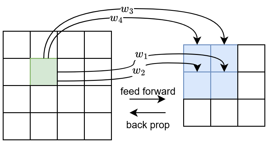
A few more words on convolutional layer. First, $$ \text{\# of parameters}=(\text{\# of input channels}\times\text{kernel size}^2+1)\times\text{\# of output channels} $$ Second, we have stride and padding for convolutional layer. If the original size of some dimension is $n$, then the output size is $$ \left\lfloor\frac{n+\text{padding}-\text{kernel}}{\text{stride}}\right\rfloor+1 $$ On backpropagation of convolutional layer, we first write convolution as, like $$ z^{(l+1,\cdot)}\gets\mat{ w_1&w_2&0&w_3&w_4&0&0&0&0\\ 0&w_1&w_2&0&w_3&w_4&0&0&0\\ 0&0&0&w_1&w_2&0&w_3&w_4&0\\ 0&0&0&0&w_1&w_2&0&w_3&w_4\\ }z^{(l,\cdot)}+\mat{b\\b\\b\\b} $$ where $W=\mat{w_1&w_2\\w_3&w_4}$ is the kernel. Since we know that, for $\b z_{l+1}=W_l\b z_l+\b b_l$, $$ \nabla_{\b z_l}\ell=\left(\frac{\p\ell}{\p\b z_l}\right)^\top=\left(\frac{\p\ell}{\p\b z_{l+1}}W_l\right)^\top=W_l^\top\nabla_{\b z_{l+1}}\ell $$ so, examine $$ \begin{align*} g^{(l,\cdot)}&=\mat{w_1&0&0&0\\ w_2&w_1&0&0\\ 0&w_2&0&0\\ w_3&0&w_1&0\\ w_4&w_3&w_2&w_1\\ 0&w_4&0&w_2\\ 0&0&w_3&0\\0&0&w_4&w_3\\ 0&0&0&w_4}g^{(l+1,\cdot)}\\ &= \mat{ w_4&w_3&0&0&w_2&w_1&0&0&0&0&0&0&0&0&0&0\\ 0&w_4&w_3&0&0&w_2&w_1&0&0&0&0&0&0&0&0&0\\ 0&0&w_4&w_3&0&0&w_2&w_1&0&0&0&0&0&0&0&0\\ 0&0&0&0&w_4&w_3&0&0&w_2&w_1&0&0&0&0&0&0\\ 0&0&0&0&0&w_4&w_3&0&0&w_2&w_1&0&0&0&0&0\\ 0&0&0&0&0&0&w_4&w_3&0&0&w_2&w_1&0&0&0&0\\ 0&0&0&0&0&0&0&0&w_4&w_3&0&0&w_2&w_1&0&0\\ 0&0&0&0&0&0&0&0&0&w_4&w_3&0&0&w_2&w_1&0\\ 0&0&0&0&0&0&0&0&0&0&w_4&w_3&0&0&w_2&w_1\\ }\mat{0\\0\\0\\0\\0\\ g^{(l+1,\cdot)}_1\\ g^{(l+1,\cdot)}_2\\0\\0\\ g^{(l+1,\cdot)}_3\\ g^{(l+1,\cdot)}_4\\0\\0\\0\\0\\0} \end{align*} $$ so we find that, backpropagation through the convolution layer is just convolution by flipped filter after padding.
Tricks
Gradient Descent
$$ \b\theta^\prime=\b\theta-\eta\nabla_{\b\theta}\ell(\b\theta) $$
For stochastic gradient descent, from mathematical point of view rather than “minibatch” point of view, $$ \b\theta^\prime=\b\theta-\eta(\nabla_{\b\theta}\ell(\b\theta)+\b\xi) $$
ReLU
Vanishing gradient problem is caused by both small derivative value of sigmoid and small (initial) parameters, while exploding gradient problem is only caused by large parameters. ReLU can only solve the small derivative problem. However, it introduces dying ReLU problem. To tackle this, people invented leaky ReLU, SiLU, etc.
Planning and RL
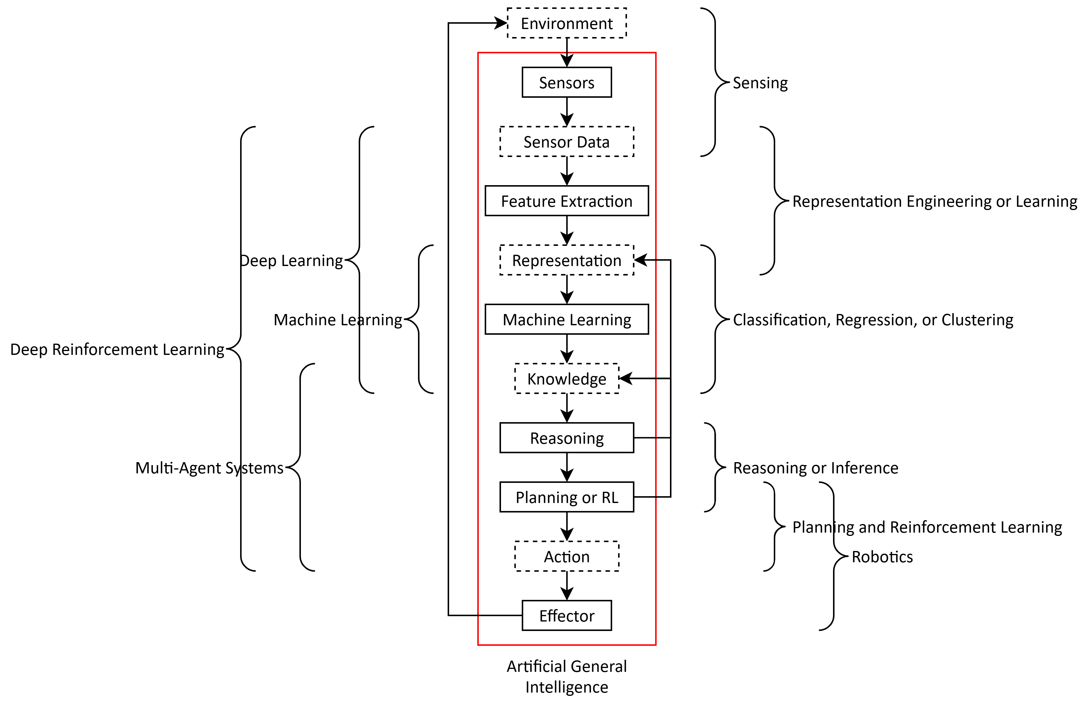
Previously, all the ML models are about producing knowledge, but now we enter the field of interacting with the environment.
Search
The simplest, deterministic way of planning, is search.
A search problem consists of state space $S$, start state $s_{\rm start}$, actions space $A$, successors (of actions), cost (of actions), and goal test. A solution is a sequence of actions that transform $s_{\rm start}$ to a state that satisfies the goal condition.
A* Search
The only reason why A* is better than BFS/Dijkstra is A* doesn’t explore all the vertices.
A* is simply Dijkstra, changing the key of $u$ in the priority queue from $d_u$ to $d_u+e_u$, where $e_u$ is the estimated distance from $u$ to the goal, and outputting the answer when some goal is extracted from the priority queue. It’s easy to see, for $e_u=0$, it’s Dijkstra; for $e_u=\operatorname{dis}(u,t)$, only the vertices on the shortest path from $s$ to $t$ (the nearest goal) will be explored.
From here we follow the convention taught in class: rename $d_u$ as $f(u)$, and $e_u$ as $h(u)$ (called a heuristic), vertices as states, and length as cost. There are three A* variants under different assumptions on $h(u)$:
- No constraint. A* might be incorrect.
- (admissible) $0\le h(u)\le h^{*}(u)$ where $h^{*}(u)=\min_{\text{goal }t}\operatorname{dis}(u,t)$. In this case some $u$ may be pushed into/popped from queue multiple times, but the lowest cost is ensured to be found because every state nearer from the start state than any goal will be expanded before the goal. We say in this case, tree search can solve the problem.
- (consistent) $h(u)\le h(v)+w(u,v)$. In this case we can prove that when $u$ is popped the first time, the cost is optimal. We say in this case, graph search can solve the problem.
Obviously consistent $\implies$ admissible. We can see the stupid heuristic as setting $w^\prime(u,v)=w(u,v)-h(u)+h(v)$, then consistency condition is just nonnegative weights. So A* is explained in one sentence, but non-TCS guys use an entire session to talk about it with vague expressions. I can’t stand it.
MDP
Definition
When facing the real world, there are uncertainties. When taking an action $a$ at state $s$, the next state is not deterministic, but follows a probability distribution, i.e. $$ \Pr[s^\prime\mid s,a]=T(s,a,s^\prime) $$ and everything else are the same as search, except the cost function is replaced by reward function $R(\text{state})$ (and the goal is to maximize it). It’s called Markov Decision Process. It has the following properties:
- First-order Markovian dynamics (history independence). $\Pr(s_{t+1}\mid s_t,a_t,s_{t-1},a_{t-1},\cdots,s_0)=\Pr(s_{t+1}\mid s_t,a_t)$.
- Reward is deterministic.
- The probability distribution does not depend on time.
- We can observe $s_{t+1}$ after it’s sampled.
Note that the first-order Markovian dynamics does not mean that the process is necessarily independent of the “history” because we can let ($\circ$ means concatenation) $$ s^\prime=s\circ a\circ\Delta\text{ w.p. }T(s,a,\Delta) $$ But usually it’s not the case in practice.
In the agent’s point of view, there’s an additional concept called “observation”. The observation space is denoted as $\Omega$, and the observation $o\in\Omega$ is determined by the action and the succeeding state: $$ \text{there is a distribution }\Pr[o\mid s^\prime,a] $$ A history $h_t$ is defined as $$ h_t=(a_0,o_1,R_1,a_1,o_2,R_2,\cdots,a_{t-1},o_t,R_t) $$ and the internal state of the agent is defined as a summary of experience $$ \text{internal state}=f(h_t) $$ and the internal state is also called $h_t$. Usually $f$ will not keep all the information. Think of, for example, LSTM. Furthermore, we call “fully observed environment”, when the true state can be inferred from the observation. In this case, clearly, we don’t need to distinguish the true state and the internal state. On the flip side, if the environment is not fully observed, we call the process a “partially observed Markov decision process” (POMDP). Then conditioned on the current internal state, the agent can form a “guess” on the true state, that is a “belief state” $b_t=b(h_t)\in\Delta(S)$.
Some real-world examples for better understanding:
- Go. Fully observed.
- Poker (德扑). The optimal decision requires you to remember past actions, bets, and the number of players who folded, etc.
- Robot navigation. If there’s a map/GPS, then it is fully observed. Otherwise, it’s partially observed and the robot needs to use its history to reduce uncertainty.
There are two types of problem:
- Planning, the dynamics model (probability distribution) is known.
- RL, not known.
Theoretical Guarantee
To solve an MDP, we want to find a policy $\pi:S\to A$ or $\pi:S\to \Delta(A)$. There are two types of policies:
- Non-stationary policy. The action also depends on the steps to go.
- Stationary policy. There are infinitely many future steps.
Note that the four properties of an MDP still hold.
For infinite horizon case, to evaluate a policy, we define a value function: $$ V_\pi(s)=\E\left(\sum_{t\ge 0}\gamma^tR(s_t)\middle|\pi,s\right) $$ or $$ V_\pi(s)=R(s)+\gamma\E(V_\pi(s^\prime)\mid s,\pi(s))\tag{Bellman equation} $$ Maybe not that ideal, just compromise on convergence.
We claim that
Theorem. $\exists\pi$, $\forall s$, $\forall \pi^\prime$, $V_\pi(s)\ge V_{\pi^\prime}(s)$, that is, such “best” policy exists.
Proof. Here we define $V_{*}$ recursively: $$ V_{*}(s)=R(s)+\gamma\max_a\E(V_{*}(s^\prime)\mid s,a) $$ Lemma. $V_{*}$ uniquely exists, and $\forall s$, $V_{*}(s)=\max_\pi V_\pi(s)$.
Then we construct $$ \pi_{*}(s)=\operatorname*{argmax}_a\E(V_{*}(s^\prime)\mid s,a) $$ Then such $\pi_{*}$ satisfies the condition.
Now we prove the lemma. Consider the Bellman operator $\B:\R^{|S|}\to\R^{|S|}$: $$ \B V(s)=R(s)+\gamma\max_a\E(V(s^\prime)\mid s,a) $$ $$ \begin{align*} \lVert\B V_1-\B V_2\rVert_{\infty} &=\gamma\max_s\left\lvert\max_a\E(V_1(s^\prime)\mid s,a)-\max_a\E(V_2(s^\prime)\mid s,a)\right\rvert\\ &\le\gamma\max_s\max_a\left\lvert\E(V_1(s^\prime)\mid s,a)-\E(V_2(s^\prime)\mid s,a)\right\rvert\\ &\le\gamma\max_s\max_a\sum_{s^\prime}\Pr[s^\prime\mid s,a]\left\lvert V_1(s^\prime)-V_2(s^\prime)\right\rvert\\ &\le\gamma\max_{s^\prime}\left\lvert V_1(s^\prime)-V_2(s^\prime)\right\rvert\\ &=\gamma\|V_1-V_2\|_{\infty} \end{align*} $$ So by the Banach fixed-point theorem, there exists unique $V_{*}$ such that $\B V_{*}=V_{*}$. Also a corollary is linear convergence.
If for some $V_\pi$, $V_\pi(s)>V_{*}(s)$, then $V_\pi$ is not a fixed point, and $\exists s^\prime$, $\B V_\pi(s^\prime)>V_\pi(s^\prime)$. If we only change $\pi(s^\prime)$, we’ll get a strictly better policy because the probability served as coefficient in the Bellman equation is nonnegative. Here we assume the policy space is finite, so we’ll reach a contradiction.
Value Iteration
Just repeatedly calculate $V$. By the Banach fixed-point theorem,
- $\|V_k-V_{*}\|\le\gamma^kR_{\max}/(1-\gamma)$
- $\|V_k-V_{k-1}\|\le\eps\implies\|V_k-V_{*}\|\le\eps\gamma/(1-\gamma)$.
- Let $V_g$ be the value of $\pi_V$ constructed by $\operatorname{argmax}$, then $\|V-V_{*}\|\le\eps\implies\|V_g-V_{*}\|\le2\eps\gamma/(1-\gamma)$.
Policy Iteration
Each iteration, compute $V_\pi$ by current $\pi$ then update $\pi$ by $V_\pi$ (still, $\operatorname{argmax}$), until $\pi$ fixes.
Since $$ \max_a\E(V_\pi(s^\prime)\mid s,a)\ge\E(V_\pi(s^\prime)\mid s,\pi(s)) $$ We can iteratively use this inequality to show $\pi^\prime$ must improve over $\pi$ (if equality holds, it means the fix-point is reached). In theory, the algorithm might run through every policy then result in exponential time, but it’s not the case in practice.
How to calculate $V_\pi$? We need to solve a linear equation system.
In short, value iteration needs more iterations than policy iteration empirically. Value iteration is $O(S^2A)$, while policy iteration is $O(S^3)$ but can be reduced to $O(kS^2)$: just like value iteration, calculate $V_\pi$ by a few iterations. This is called modified policy iteration.
Other Tricks
- In-place value iteration. Every time randomly choose an $s$ and update $V(s)$.
- Prioritized sweeping. Every time select $s$ s.t. $\delta(s)=\left\lvert R(s)+\max_a\E(V(s^\prime)\mid s,a)-V(s)\right\rvert$ is the largest. Need to reversely update those $\delta(s_{\rm pre})$ such that $\Pr[s\mid s_{\rm pre},a_{\rm best}]>0$. Use priority queue to maintain.
- Run the policy, use agent’s experience to guide the selection of $s$.
- When $V$ requires too much memory, we can use NN to fit $V$.
MDP Variations
- Infinite MDP: countably infinite states/actions; continuous state/action; continuous time.
- POMDP: can be reduced to an (infinite) history tree, or an continuous MDP with belief states.
- Ergodic MDP. A few words is needed here.
An ergodic MP is an irreducible, aperiodic MP. An ergodic MDP is an MDP whose MP induced by any policy is ergodic. By 计智应数, an ergodic MP has a unique stationary distribution. Thus the following quantity is well-defined w.r.t. a policy $\pi$: $$ \rho_\pi=\lim_{T\to\infty}\frac1T\E\left(\sum_{t=1}^TR_t\right) $$ it’s called the average reward per time-step.
The value function of an undiscounted ($\gamma=1$), ergodic MDP can be expressed in terms of average reward. $$ \tilde V_\pi(s)=\E\left(\sum_{t\ge 1}(R_t-\rho_\pi)\middle| s_0=s\right) $$ by theory of mixing time, $R_t-\rho^\pi=\Omicron(\lambda^t)$ for some $0<\lambda<1$, so the infinite sum converges.
Bellman equation form: $$ \tilde V_\pi(s)=\E((R^\prime-\rho_\pi)+\tilde V_\pi(s^\prime)\mid s) $$
Reinforcement Learning
RL is MDP, minus the knowledge about transition $T$ and/or reward $R$.
In RL, a learning algorithm is called an agent. There are two main attributes of an agent that we differentiate, that are:
- Passive learning vs. active learning. Passive learning is just following a fixed policy, and try to estimate the utility of the policy $V_\pi(\cdot)$. Active learning select the policy. While it aims at finding the optimal policy, it utilize the current policy to explore, that is, gaining information about the MDP that guides the further policy selection.
- Model-based vs. model-free. A model-based agent explicitly stores a representation of $T$ and $R$, then the overall problem is more like MDP previously introduced, and may be solved by, e.g. policy iteration. A model-free agent learns $V$ or $\pi$ directly from trial-and-error experience with the environment, without explicitly learning the model (MDP).
| Model-Free | Model-Based | |
|---|---|---|
| Passive Learning | MC | ADP, TD |
| Active Learning | Q-Learning, SARSA, DQN, PPO, SAC | Dyna-Q |
Passive Learning
From here on, $T$, $R$, and $V$ all refer to estimated values; formally they should be written as $\hat T$, $\hat R$, and $\hat V$.
Now a policy $\pi$ to be evaluated is given.
- Direct estimation, or Monte Carlo (MC). Just run a lot of episodes (each time act according to $\pi$ until a terminal state is reached), and average reward-to-go. It converges but very slowly. It doesn’t utilize Bellman equation.
- Adaptive dynamic programming (ADP). It follows $\pi$ for a while, to get $T$ and $R$, then solve for $V_\pi(\cdot)$. Correctness: can bound error with Chernoff bounds.
- Temporal difference learning (TD). The idea is to do local updates of the value function on a per-action basis, instead of learning the model and solving the Bellman equation at the end. Details are as follows:
Consider updating the value function in some way: $$ V_\pi^\prime(s)\gets\begin{cases}V_\pi(s)&(\text{old})\\R(s)+\gamma\E(V_\pi(s^\prime)\mid s,\pi(s))&(\text{new})\end{cases} $$ Here $\text{new}$ is obtained by sampling: $$ \text{new}=R(s)+\gamma V_\pi(s^\prime),s^\prime\sim T(s,\pi(s),\cdot) $$ so that $\E(\text{new})=R(s)+\gamma\E(V_\pi(s^\prime)\mid s,\pi(s))$.
To guarantee some kind of stability, we set a “learning rate” $\alpha$, then $$ V_\pi^\prime(s)=(1-\alpha)(\text{old})+\alpha(\text{new}) $$ Thus $$ V^\prime_\pi(s)=V_\pi(s)+\alpha(R(s)+\gamma V_\pi(s^\prime)-V_\pi(s)) $$ With appropriately decreasing $\alpha$, one can prove convergence.
Active Learning
Now we need to find a good policy $\pi$.
There’s a main challenge called the Exploration-Exploitation Dilemma.
- MC-based naïve approach. Explore (take random action each time) for a long long time to learn $T$ and $R$, then turn the problem into MDP problem. This is one extreme of complete exploration.
- ADP-based naïve approach. Every cycle, follow the policy $\pi$ solved by the previous cycle for a while and estimate $T$ and $R$, then compute $V_\pi$ by the gained information. Finally compute the new policy $\pi^\prime$ by $\argmax$. This is the other extreme of complete exploitation. It is usually incorrect because it can easily get stuck in local minima.
GLIE
We can modify “following the previously obtained greedy policy” to avoid getting stuck:
- Each step with probability $1-p(t)$ select the greedy action, and with probability $p(t)$ act randomly. $p(t)=1/t$.
- Select action according to Boltzmann distribution $\Pr[a\mid s]=\exp(Q(s,a)/T)/\sum_{a^\prime}\exp(Q(s,a^\prime)/T)$.
- Optimistic exploration. Assign the highest possible value to any state-action pair that has not been explored enough. Under this framework, there is an algorithm called $\text{Rmax}$. Specifically, it redirects the transition of any state-action pair that has been visited fewer than $N_e$ times to itself and sets the reward to $R_{\max}$ (so its $Q$ value is $V_{\max}=R_{\max}/(1-\gamma)$). $\text{Rmax}$ has a theoretical convergence guarantee called a PAC guarantee.
These exploration policies are all so-called GLIE, greedy in the limit of infinite exploration.
Q-Learning
Notice that there comes a new value function $Q$: $$ Q(s,a):=R(s)+\gamma\E\left(\max_{a^\prime}Q(s^\prime,a^\prime)\middle|s,a\right) $$ It’s especially useful for optimizing TD-based active RL. When trying to analogize TD-based active RL to ADP-based active RL, it seems like the only thing to be changed is the updating process of $V_\pi$. However the greedy policy requires $\argmax_a\set{\cdots}$, where $T$ and $R$ are needed. So TD-based active RL is no longer model-free. In order to prevent learning the model, we should directly estimate $Q$ instead of $V_\pi$. This leads to Q-learning. The updating step of $Q$ is similar to that in TD: $$ Q^\prime(s,a)=Q(s,a)+\alpha\left(R(s)+\gamma\max_{a^\prime}Q(s^\prime,a^\prime)-Q(s,a)\right) $$
With the same exploration policy such as Boltzmann exploration, one can prove that with learning rate satisfying $\sum\alpha_n=\infty\land\sum\alpha_n^2<\infty$, Q-learning converges to the true, optimal $Q$ function.
For goal-based problems where the big reward appears only in the goal state, in each episode only one more $Q(s,a)$ can see that big reward. To accelerate convergence, we can use optimizations that look like “back-propagation”, including trajectory replay and reverse updates.
SARSA
Now consider another pair of attributes:
- Off-policy vs. on-policy. If the policy used to select the action and the policy used to evaluate the next action are the same, then such agent is called on-policy, otherwise it’s called off-policy. Q-learning is obviously off-policy, because it follows a mixture of greedy action and random action when deciding the next step (exploring), while it chooses $\max_{a^\prime}Q$ when calculating $Q$ function (exploiting).
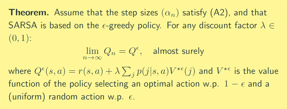
State-Action-Reward-State-Action (SARSA) is an on-policy type of agent similar to Q-learning. The only difference is that, after the update: $$ Q^\prime(s,a)=Q(s,a)+\alpha\left(R(s)+\gamma Q(s^\prime,a^\prime)-Q(s,a)\right)\text{ where }a^\prime=\begin{cases}\argmax_{a^\prime}Q(s^\prime,a^\prime),&\text{w.p. }1-\epsilon\\ \text{an action uniformly at random},&\text{w.p. }\epsilon\end{cases} $$ The action taken (giving $s^{\prime\prime}$) is exactly $a^\prime$. Notice that in Q-learning, the $a^\prime=\argmax Q$ used for update is not necessarily the actual action leading the trajectory.
Also it’s almost the same as the first exploration strategy in ADP-based learning, except that $\epsilon$ is a fixed constant.
SARSA learns safer policy than Q-learning. This behavior significantly manifests in the classical cliff walking problem. An easy way to understand that is to regard the $\epsilon$-greedy policy as the agent itself occasionally loses its mind and does some crazy decisions, so in order to prevent catastrophic negative reward it tends to choose a safer pathway.
Note that when I say “SARSA learns safer policy”, I refer to “the output policy” of SARSA, which is still a deterministic policy obtained by taking $\pi(s)=\argmax_aQ(s,a)$.
| MC Passive | ADP Passive | TD Passive | MC Active | ADP Active | TD Active | Q-Learning | SARSA | |
|---|---|---|---|---|---|---|---|---|
| Time/it | ? | $O(kS^2)$ | $O(1)$ | ? | $O(kS^2)$ | $O(1)$ | $O(1)$ | $O(1)$ |
| Space | $O(S^2A)$ | $O(S^2A)$ | $O(S^2A)$ | $O(S^2A)$ | $O(S^2A)$ | $O(SA)$ | $O(SA)$ | |
| Model | based | based | free | based | based | based | free | free |
Deep Reinforcement Learning
RL with Function Approximation
When solving real-world RL problems, we can’t afford to store the full tabular $V$ or $Q$. So we consider approximating them using kernel methods or linear approximation. Define a set of features $f_1(s)\sim f_n(s)$, and $$ V_\theta(s)=\theta_0+\sum_{i=1}^n\theta_if_i(s) $$ Now first we consider model-based TD. The expected “correct” $V$ is $v(s)=R(s)+\gamma V_\theta(s^\prime)$, and the current value is $V_\theta(s)$. Directly using GD with quadratic loss function, the gradient update should be $$ \theta^\prime=\theta-\alpha\nabla_\theta\left(\frac12\left(v(s)-\theta_0-\sum_{i=1}^n\theta_if_i(s)\right)^2\right)=\theta+\alpha(R(s)+\gamma V_\theta(s^\prime)-V_\theta(s))\mat{1\\f(s)} $$ For model-free TD, it’s also basically identical to Q-learning: $$ Q_\theta(s,a)=\theta_0+\sum_{i=1}^n\theta_if_i(s,a) $$
$$ \theta^\prime=\theta+\alpha\left(R(s)+\gamma\max_{a^\prime}Q_\theta(s^\prime,a^\prime)-Q_\theta(s,a)\right)\mat{1\\f(s,a)} $$
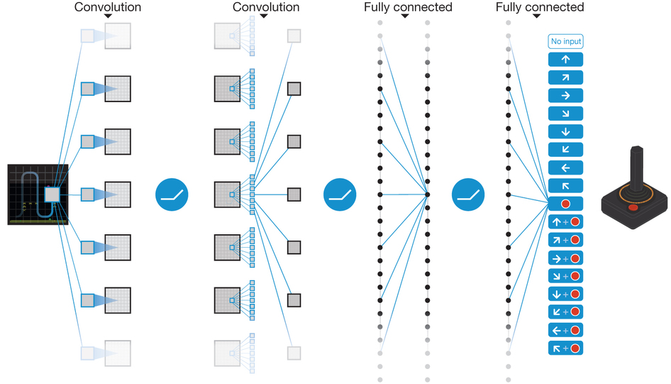
Furthermore, why not use NN to approximate $Q$? (the convergence is not guaranteed, though) This leads to Deep Q-Networks, i.e. DQN.
Stability Problem and Solutions
Naïve Q-learning on DNNs (with the past few frames as input) oscillates or diverges because the data is sequential and successive samples are correlated, and also correlated with the taken action. Since the loss landscape of DNNs is complicated, the policy may oscillate (between several behavior modes). Also, because there are unstable gradient issues, we need to tune hyperparameters carefully. But there’re many different environment conditions. There’re several tricks that make it more stable:
- Experience replay. This is to remove correlations. Do not use the most recent observed transitions, but store millions of transitions in replay memory $D$. Every time sample mini-batches from it and optimize.
- Fixed target Q-Network. So we want $R(s)+\gamma\max_{a^\prime}Q_\theta(s^\prime,a^\prime)=Q_{\theta^\prime}(s,a)\cdots(*)$. Previously we make recurrently update to minimize the loss, and in the next step, the reference $Q$ is changed to $Q_{\theta^\prime}$. Now we fix the reference $\theta$ (in LHS of $(*)$) for thousands of steps and optimize $\theta^\prime$.
- Control the reward/value range like clipping to $[-1,+1]$.
By 1 and 2, the optimization target is changed to: $$ \begin{array}{c} \min.\left(R(s)+\gamma\max_{a^\prime}Q_{\theta_t}(s^\prime,a^\prime)-Q_{\theta_{t+1}}(s,a)\right)^2\\ \downarrow\\ \min.\E_{(s,a,r,s^\prime)\sim U(D)}\left(r+\gamma\max_{a^\prime}Q_{\theta_t}(s^\prime,a^\prime)-Q_{\theta_{t+1}}(s,a)\right)^2\\ \downarrow\\ \min.\E_{(s,a,r,s^\prime)\sim U(D)}\left(r+\gamma\max_{a^\prime}Q_{\theta_{\lfloor t/T\rfloor T}}(s^\prime,a^\prime)-Q_{\theta_{t+1}}(s,a)\right)^2 \end{array} $$
Maximization Bias and Double Q-Learning
Another problem is called the maximization bias. Recall the update formula of tabular Q-learning: $$ Q^\prime(s,a)=Q(s,a)+\alpha\left(R(s)+\gamma\max_{a^\prime}Q(s^\prime,a^\prime)-Q(s,a)\right) $$ One can see that $$ \E\left(\max_ix_i\right)\ge\E(x_{*})=\max_i\E(x_i) $$ so with randomness (even the previous $Q$ has unbiased noise), $Q$ will be overestimating. The solution is double Q-learning: Train two $Q$ functions, every time randomly choose one to update, like $$ Q_1^\prime(s,a)=Q_1(s,a)+\alpha\left(R(s)+\gamma Q_2(s^\prime,\argmax_{a^\prime}Q_1(s^\prime,a^\prime))-Q_1(s,a)\right) $$ It can be proven that under some assumptions, it underestimates. But the key is that because of the $\max$, underestimation is less damaging than overestimation, since the latter leads to a feedback loop, but the former cannot.
When determining the next action, take $\argmax$ over $Q_1+Q_2$.
The same idea can be applied to DQN. Here the old Q-network can be used as $Q_2$:
$$
\min.\left(r+\gamma Q_{\theta_{\text{old}}}(s^\prime,\argmax_{a^\prime}Q_\theta(s^\prime,a^\prime))-Q_\theta(s,a)\right)^2
$$
Combined with experience replay, here’s another trick: for multiple past experiences $\set{(s,a)}$, choose among them according to the above quadratic error, like
$$
P(i)=\frac{\mathrm{err}_i^\alpha}{\sum_k\mathrm{err}_k^\alpha}
$$
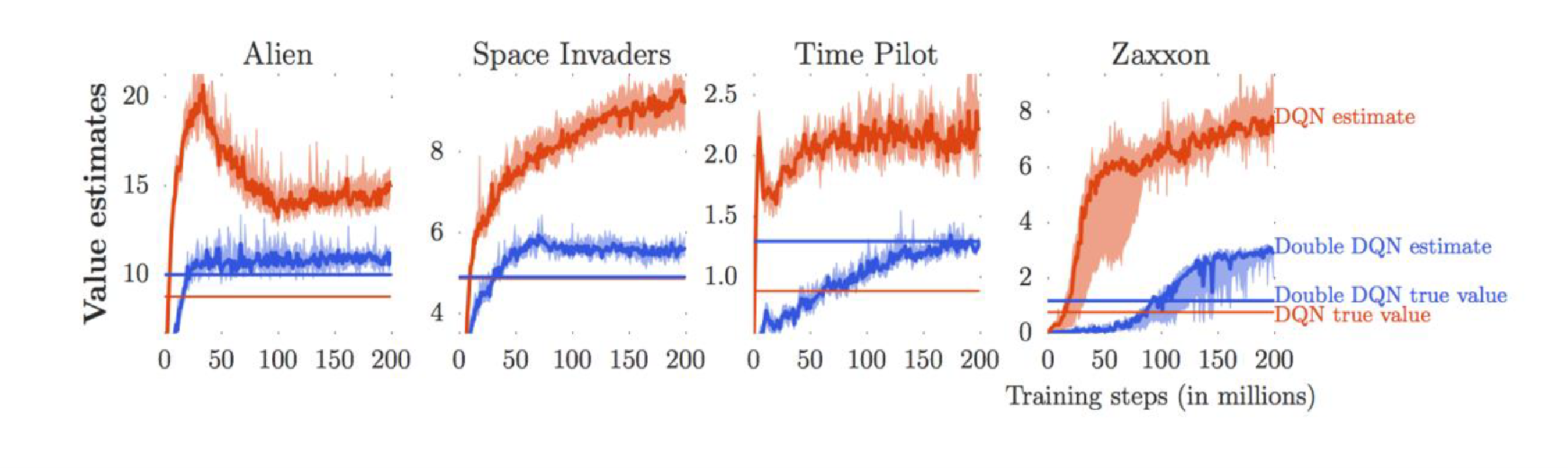
This plot shows that double DQN is less biased and has lower variance. Note that the “true value” is $\E(\sum\gamma^tr_t)$ when following the policy yielded by $\argmax$.
Policy-Based RL
Instead of learning $V$ or $Q$ by simulating some policy for a huge number of steps, policy-based RL methods directly learn the model that determine the actions, that is, $\pi_\theta(s,a)=\Pr[a\mid s;\theta]$, learn $\theta$ by GD.
There’re a few intuitive reasons:
- Often the feature-based policies that work well aren’t the ones that approximate $V$/$Q$ best.
- The final goal of RL is finding a good policy, which can be achieved by only getting the ordering of $Q$ values right. But Q-learning prioritizes getting $Q$ values close.
- $V$ or $Q$ leads to deterministic (or near-deterministic like $\epsilon$-greedy) policies, while in some problems, mixed strategy is the optimal.
The advantages of policy-based RL:
- Better convergence properties: $\pi_\theta(s,a)$ changes continuously, unlike the $\argmax$ of value-based RL changing suddenly.
- Effective in high-dimensional or continuous action spaces.
- Can learn stochastic policies.
Disadvantages:
- Typically converge to a local optimum.
- Evaluation of the policy has high variance, resulting in slow convergence.
Objectives
We assume the Markov process induced by the policy $\pi_\theta$ is ergodic, so that there exists a unique stable distribution $d_{\pi_\theta}(\cdot)$.
- In episodic environments like video games, the starting state matters. So we consider $J_1(\theta)=V_{\pi_\theta}(s_0)$.
- In continuing environments we consider the limit value $J_{\rm avV}(\theta)=\sum_sd_{\pi_\theta}(s)V_{\pi_\theta}(s)$.
- However if we want $\gamma=1$ then $J_{\rm avV}$ is not available. Consider $J_{\rm avR}(\theta)=\sum_sd_{\pi_\theta}(s)\sum_a\pi_\theta(s,a)R(s,a)$. When $\gamma<1$, $J_{\rm avV}=\frac{1}{1-\gamma}J_{\rm avR}$.
Finite Difference Policy Gradient
Compute $$ \frac{\p J(\theta)}{\p\theta_i}\approx\frac{J(\theta+\epsilon e_i)-J(\theta)}{\epsilon} $$ Stupid.
REINFORCE
Here we assume the reward depends on the state and the action.
The motivation is to “sample the gradient”. To do that, extracting a $\pi_\theta(s,a)$ term from the gradient is favorable. Starting with $\nabla_\theta\pi_\theta(s,a)$: $$ \nabla_\theta\pi_\theta(s,a)=\pi_\theta(s,a)\nabla_\theta\log\pi_\theta(s,a) $$ An easy case is the first step. Suppose $s_0\sim d(\cdot)$: $$ \nabla_\theta\E(R(s_0,a_0))=\nabla_\theta\sum_sd(s)\sum_a\pi_\theta(s,a)R(s,a)=\sum_sd(s)\sum_a\pi_\theta(s,a)\nabla_\theta\log\pi_\theta(s,a)R(s,a)=\E\left(\nabla_\theta\log\pi_\theta(s,a)R(s,a)\right) $$ The key point is, $\nabla_\theta\E$ cannot be calculated by sampling, while $\E(\nabla_\theta)$ can, because $\pi_\theta(s,a)$ is usually produced by an NN, thus $\nabla_\theta\log\pi_\theta(s,a)$ can be analytically computed.
Now, $$ \begin{align*} \nabla_\theta V_{\pi_\theta}(s)&=\nabla_\theta\left(\sum_a\pi_\theta(s,a)\left(R(s,a)+\gamma\sum_{s^\prime}\Pr[s^\prime\mid s,a]V_{\pi_\theta}(s^\prime)\right)\right)\\ &=\sum_a\nabla_\theta\pi_\theta(s,a)\left(R(s,a)+\gamma\sum_{s^\prime}\Pr[s^\prime\mid s,a]V_{\pi_\theta}(s^\prime)\right)+\sum_a\pi_\theta(s,a)\gamma\sum_{s^\prime}\Pr[s^\prime\mid s,a]\nabla_\theta V_{\pi_\theta}(s^\prime)\\ &=\sum_a\nabla_\theta\pi_\theta(s,a)Q_{\pi_\theta}(s,a)+\gamma\sum_{s^\prime}\Pr[s^\prime\mid s]\nabla_\theta V_{\pi_\theta}(s^\prime)\\ &=\cdots\\ &=\sum_t\gamma^t\sum_{s^\prime}\Pr[s^\prime\mid s;\text{after }t\text{ steps}]\sum_a\nabla_\theta\pi_\theta(s,a)Q_{\pi_\theta}(s,a) \end{align*} $$
$$ \begin{align*} \nabla_\theta J_1(\theta)&=\sum_sd(s)\nabla_\theta V_{\pi_\theta}(s)\\ &=\sum_sd(s)\sum_t\gamma^t\sum_{s^\prime}\Pr[s^\prime\mid s;\text{after }t\text{ steps}]\sum_a\nabla_\theta\pi_\theta(s,a)Q_{\pi_\theta}(s,a)\\ &=\sum_t\gamma^t\sum_{s^\prime}\Pr[s_t=s^\prime]\sum_a\nabla_\theta\pi_\theta(s,a)Q_{\pi_\theta}(s,a)\\ &=\sum_s\left(\sum_t\gamma^t\Pr[s_t=s]\right)\left(\sum_a\nabla_\theta\pi_\theta(s,a)Q_{\pi_\theta}(s,a)\right) \end{align*} $$
If we define discounted visitation distribution $$ d_{\pi_\theta}^\prime(s)\propto\sum_t\gamma^t\Pr[s_t=s] $$ we get $$ \nabla_\theta J_1(\theta)=\frac{1}{1-\gamma}\E_{s\sim d_{\pi_\theta}^\prime(\cdot)}\left(\sum_a\nabla_\theta\pi_\theta(s,a)Q_{\pi_\theta}(s,a)\right)=\frac1{1-\gamma}\E_{s\sim d_{\pi_\theta}(\cdot),a\sim \pi_\theta(s,\cdot)}\left(\nabla_\theta\log\pi_\theta(s,a)Q_{\pi_\theta}(s,a)\right) $$ Actually it’s the Policy Gradient Theorem: For any differentiable policy $\pi_\theta(s,a)$, $$ \nabla_\theta J(\theta)=\E\left(\nabla_\theta\log \pi_\theta(s,a)Q_{\pi_\theta}(s,a)\right) $$ This holds for any of the choices $J=J_1,J_{\rm avR},\frac1{1-\gamma}J_{\rm avV}$. For $J_1$, the $1/(1-\gamma)$ coefficient is gotten rid of by forcing $d_{\pi_\theta}(s)=\sum_t\gamma^t\Pr[s_t=s]$ (So it’s notation abuse since now $\E$ doesn’t really denote expectation). For $J_{\rm avR}$ and $\frac1{1-\gamma}J_{\rm avV}$, $d_\pi$ is just the stationary distribution, while $Q$ is changed to differential Q-value: $$ Q_{\pi_\theta}^\prime(s, a)=R(s,a)-J_{\rm avR}(\theta)+\E(Q_{\pi_\theta}^\prime(s^\prime,a^\prime)) $$ The proof from Gemini is here.
So the final algorithm is just $\theta\xleftarrow{+}\alpha v_t\nabla_\theta\log\pi_\theta(s_t,a_t)$ following a sampled trajectory. Here $v_t$ is the reward-to-go.
Actor-Critic Methods
Recall that value-based and policy-based RL each have their own advantages and disadvantages. How about composing them together?
The critic is a network parameterized by $\phi$, denoted $Q_\phi(s,a)$.
The actor is the same as above, $\pi_\theta(s,a)$.
Following a trajectory, the parameters are updated: $$ \theta\xleftarrow{+}\alpha Q_\phi(s_t,a_t)\nabla_\theta\log\pi_\theta(s_t,a_t) $$
$$ \phi\xleftarrow{+}\beta(R(s_t,a_t)+\gamma Q_\phi(s_{t+1},a_{t+1})-Q_\phi(s_t,a_t))\nabla_\phi Q_\phi(s_t,a_t) $$
You might have already caught the questionable point: this doesn’t conform to any version ($J_1,J_{\rm avR},\frac1{1-\gamma}J_{\rm avV}$) of the Policy Gradient Theorem! By Gemini, the objective is another variant, called the average performance with discounted Q-values: $$ J_{\text{hybrid}}(\theta) = \E_{s \sim d_\pi(\cdot)} (V_\pi(s)) $$ Forget about it.
Now we aim to reduce the variance of $\nabla_\theta\log \pi_\theta(s,a)Q_{\pi_\theta}(s,a)$. Notice that for any function only of $s$: $$ \E(\nabla_\theta\log \pi_\theta(s,a)B(s))=\sum_sd_{\pi_\theta}(s)\sum_a\nabla_\theta\pi_\theta(s,a)B(s)=\sum_sd_{\pi_\theta}(s)\nabla_\theta B(s)=0 $$ We can choose $B(s)=\E(Q(s,a))$, so $$ \nabla_\theta J(\theta)=\E\left(\nabla_\theta\log \pi_\theta(s,a)(Q_{\pi_\theta}(s,a)-V_{\pi_\theta}(s))\right) $$ to reduce the variance. Notice that it’s just the advantage function $A_{\pi_\theta}(s,a)$. This leads to some elegant update formulas: $$ \delta=R(s_t,a_t)+\gamma V_\phi(s_{t+1})-V_\phi(s_t) $$
$$ \theta\xleftarrow{+}\alpha\delta\nabla_\theta\log\pi_\theta(s_t,a_t) $$
$$ \phi\xleftarrow{+}\beta\delta\nabla_\phi V_\phi(s_t) $$
Similar to Q-learning, we’re also worried about bias in the algorithm. There’s a theorem for this:
If $\nabla_\phi Q_\phi(s,a)=\nabla_\theta\log\pi_\theta(s,a)$ and $\phi$ minimizes the error $\eps=\E(Q_{\pi_\theta}(s,a)-Q_\phi(s,a))^2$ then $$ \nabla_\phi\eps=0\implies\E((Q_{\pi_\theta}(s,a)-Q_\phi(s,a))\nabla_\phi Q_\phi(s,a))=0\implies\E(Q_{\phi}(s,a)\nabla_\theta\log\pi_\theta(s,a))=\E(Q_{\pi_\theta}(s,a)\nabla_\theta\log\pi_\theta(s,a)) $$ Obviously the minimal $\eps$ cannot be rigorously achieved, but the first condition is easy: train a feature-learning network that learns $\Phi(s,a)$, and let $\log\pi_\theta(s,a)=\theta^\top\Phi(s,a)$ and $Q_\phi(s,a)=\phi^\top\Phi(s,a)$.
Inference
I’m just leaving a catalog here since this part is easy and I have no more time.
- Definition of conditional independence
- Definition of a Bayesian net, and the equivalence of different characterizations
- Inference by join and elimination
- D-separation (the hardest)
- Sampling methods
- Inference on MMs and HMMs
- Forward algorithm & forward-backward algorithm
- Particle filtering